The Fermion Sign Problem: Why 2D Hubbard Is Unsolved

The Mott and DMFT pages kept ending at the same wall: the two-dimensional Hubbard model — the minimal model of the cuprate superconductors — is unsolved, and the reason has a name. It is not that the model is subtle to write down or that no method touches it. It is that the one method which is otherwise exact and unbiased for quantum many-body systems, quantum Monte Carlo, is defeated by a single number that shrinks exponentially: the average sign. This page builds a real determinant QMC on clusters small enough to enumerate by brute force — no Monte Carlo noise, every number exact — watches the sign hold at one where the physics protects it, and watches it collapse the moment frustration switches the protection off. That collapse, extrapolated to the systems people actually care about, is why the doped Hubbard model has resisted forty years of computing.

Where the sign comes from

Monte Carlo integrates by sampling: write a quantity as $⟨A⟩={\sum }_{c}W(c)A(c)/{\sum }_{c}W(c)$ over configurations $c$, draw configurations with probability proportional to $W(c)$, and average. It works because $W(c)$ is a probability — non-negative. For fermions it is not. Antisymmetry — the minus sign an electronic wavefunction picks up when two particles swap — leaks into the weights, and some $W(c)$ come out negative. A negative probability is meaningless, so you do the only thing you can: sample the absolute values $|W(c)|$ and carry the sign as an observable,

Everything now rides on that denominator. The average sign is a ratio of two partition functions — the physical one $Z$ and the fictitious "bosonic" one $Z_{|W|}$ built from the absolute weights — so it is an exponential of their free-energy difference:

$\Delta f$ is a free-energy density difference, strictly positive whenever the sign is not identically one, so the average sign falls off exponentially in $\beta N$ — inverse temperature times system size. And the statistical error on any measured quantity scales as $1/(⟨\mathrm{sgn}⟩\sqrt{M})$ for $M$ samples. To hold the error bar fixed while $⟨\mathrm{sgn}⟩$ halves, you must quadruple the sampling. Push to low temperature or large size and the cost grows exponentially. That is the sign problem: not a failure of cleverness but a variance that explodes faster than any polynomial amount of computing can absorb.

A determinant QMC you can enumerate by hand

Determinant QMC turns the interacting problem into free fermions moving in a fluctuating field. Trotter-decompose $e^{-\beta H}$ into imaginary-time slices; on each slice, decouple the Hubbard $U$ with a Hubbard–Stratonovich transformation that trades the two-body interaction for a discrete auxiliary spin field $s_{i,l}=\pm 1$ coupled to the electrons. At fixed field the electrons are non-interacting, and tracing them out gives a weight that is a product of two determinants, one per spin:

A production code samples the fields $s$. On a small cluster we can do better and enumerate all $2^{L{L}_{\tau }}$ of them, making the average sign an exact number rather than a noisy estimate — the cleanest possible way to see the problem, with the Monte Carlo taken out of it.

# Determinant QMC weight for a Hubbard cluster, by EXACT field enumeration.
# Trotter-split e^{-beta H}, decouple U with a discrete Hubbard-Stratonovich spin
# field s_{i,l} = +/-1, trace out the (now free) fermions -> a product of two
# determinants per field configuration. We sum over ALL 2^(L*L_tau) fields, so
# there is no Monte Carlo noise: every <sgn> below is exact.

def dqmc_enumerate(L, t, U, mu, beta, Ltau):
    dtau = beta / Ltau
    eK  = expm(-dtau * K_matrix(L, t, mu))          # free hopping propagator
    lam = np.arccosh(np.exp(dtau * U / 2))          # HS coupling: cosh(lam)=e^{dtau U/2}
    I, Wsum, absWsum = np.eye(L), 0.0, 0.0
    for bits in product((1, -1), repeat=L * Ltau):  # every auxiliary-field config
        s = np.array(bits, float).reshape(Ltau, L)
        W = 1.0
        for sigma in (1.0, -1.0):                    # up sees +lam*s, down sees -lam*s
            B = I.copy()
            for l in range(Ltau):
                B = eK @ (np.exp(sigma * lam * s[l])[:, None] * B)
            W *= np.linalg.det(I + B)                # <- can be NEGATIVE: the sign
        Wsum += W;  absWsum += abs(W)
    return Wsum / absWsum                            # <sgn> = Z / Z_|W|

Two checks gate the physics before any sign is trusted. First, on a bipartite lattice at half filling the weight is provably non-negative — particle–hole symmetry ties the two determinants together so their product never goes below zero — and the code returns $⟨\mathrm{sgn}⟩=1$ to machine precision. Second, the determinant partition function, with its Hubbard–Stratonovich prefactor restored, converges to the exact $\mathrm{Tr}{e}^{-\beta H}$ from diagonalization as the Trotter step shrinks, with the expected $\mathcal{O}(\Delta {\tau }^2)$ error:

Determinant QMC by exact field enumeration (Hubbard, U=4, t=1):

  validation
    half filling, bipartite:  <sgn> = 1.00000000   (L=2 and L=4, exact)
    Z_DQMC -> Tr e^{-beta H} as dtau -> 0:
        dtau=1.00   ratio 1.972
        dtau=0.50   ratio 1.264
        dtau=0.33   ratio 1.116
        dtau=0.25   ratio 1.065      (Trotter error ~ dtau^2 -> 0)

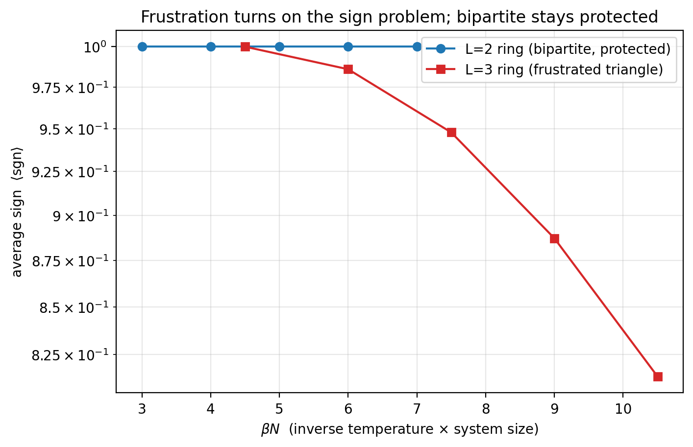
  frustration turns the sign problem ON  (half filling, mu=0)
    L=2 ring (bipartite):   <sgn> = 1.000000  at every beta      -> protected
    L=3 ring (triangle):    beta*N =  6.0    <sgn> = 0.986
                            beta*N =  7.5    <sgn> = 0.948
                            beta*N =  9.0    <sgn> = 0.887
                            beta*N = 10.5    <sgn> = 0.814        -> collapsing

Frustration switches the protection off

Here is the sign problem being born. Both systems are at half filling, so nothing is doped; the only difference is geometry. The bipartite two-site ring keeps $⟨\mathrm{sgn}⟩=1$ at every temperature — the particle–hole argument holds, every weight is non-negative, QMC would run forever without trouble. The frustrated triangle — three sites, an odd ring, the smallest lattice on which antiferromagnetic bonds cannot all be satisfied at once — is not bipartite, the protection evaporates, and the average sign slides from one down through $0.99,0.95,0.89,0.81$ as $\beta N$ grows. Extend that curve to the low temperatures where ground-state physics lives and it heads for zero. The exact same frustration that makes the triangular antiferromagnet on the quantum magnetism page a candidate spin liquid is what makes it unreachable by sign-free QMC. Frustration and the sign problem are two names for one fact.

The two ways in, and why 2D Hubbard sits in the crossfire

The protection that keeps $⟨\mathrm{sgn}⟩=1$ has two ways to fail. Frustration — a non-bipartite lattice — is the one small enough to enumerate, and it is what the figure shows. Doping is the other: pull a bipartite lattice away from half filling and the particle–hole symmetry that paired the two determinants is gone. On clusters this small the doped case stays sign-free — finite size protects it, and a real doped-Hubbard sign problem only switches on at the larger sizes and lower temperatures that exact enumeration cannot reach — but it is the more consequential failure, because the cuprate superconductors are doped Mott insulators. The two-dimensional Hubbard model at finite doping and low temperature sits exactly where every knob is turned to worst case: large $N$, small $T$, no bipartite protection. That is the unsolved problem. DMFT, the previous page, dodges it by mapping the lattice to a single impurity — but the price was throwing away the momentum dependence, and restoring it with cluster methods walks straight back into the sign problem in the cluster solver.

No universal cure — and the ways people cope

The sign problem is not merely unsolved; it is provably hard. Troyer and Wiese showed in 2005 that a general, polynomial-time cure would let you solve NP-complete problems in polynomial time — so, short of a revolution in complexity theory, no universal fix exists. What does exist is a catalogue of ways around specific instances:

• Find the sign-free corner — half filling on bipartite lattices, the attractive Hubbard model, and whole designed classes of "sign-free" Hamiltonians run exactly. Much of what is rigorously known about correlated fermions lives in these islands.
• Change the representation — the sign is basis-dependent, not physical. A clever choice of auxiliary field or worldline mapping can remove a sign that looked fatal; a lot of QMC craft is exactly this hunt.
• Accept a controlled bias — constrained-path and fixed-node QMC forbid the sign-changing moves, trading an exact-but-impossible calculation for an approximate-but-feasible one whose error you try to bound.
• Use a different method entirely — tensor networks have no sign problem (they never sample), and own one dimension outright; their two-dimensional versions are the leading sign-free attack on the 2D Hubbard model. Cold-atom quantum simulators sidestep it by letting real fermions do the computation.

Reproduce it

scripts/gen_sign_problem.py builds the determinant weight from the Hubbard–Stratonovich decoupling, enumerates every auxiliary-field configuration, and reports the exact average sign. Two validations gate it: $⟨\mathrm{sgn}⟩=1$ on bipartite half-filled clusters, and $Z_{\mathrm{DQMC}}\to \mathrm{Tr}{e}^{-\beta H}$ against full diagonalization as $\Delta \tau \to 0$. Only then does the frustrated-triangle collapse — $⟨\mathrm{sgn}⟩$ from $1$ to $0.81$ as $\beta N$ grows — carry weight. The enumeration caps the reach at a handful of sites and time slices; everything past that is the exponential wall this page is about.