Quantum Magnetism: Superexchange and the Heisenberg Chain

Take the Hubbard model and turn the repulsion $U$ up until electrons can barely move: at half filling every site is pinned to one electron, because putting two anywhere costs $U$. The charges freeze — that is a Mott insulator — but the spins do not. Each localized electron still carries a spin-½, and those spins talk to each other through a subtle, purely quantum-mechanical channel. Magnetism, here, is not a magnetic force at all. There is no dipole–dipole coupling worth mentioning; the interaction is electrostatic repulsion plus the Pauli principle, conspiring through virtual motion. This page derives that coupling — superexchange — watches the Hubbard model become the Heisenberg antiferromagnet on the nose, and then solves the resulting spin chain by exact diagonalization against the Bethe-ansatz answer known since 1931.

Why frozen charges still order their spins

Put two spins on neighboring sites in the large-$U$ Hubbard model and ask what second-order perturbation theory does with the hopping $t$. An electron can virtually hop to its neighbor and back, lowering the energy — but only if the two spins are antiparallel. If they are parallel, the Pauli principle forbids the doubly-occupied intermediate state, and the energy gain is lost. Antiparallel alignment is rewarded; the spins order antiferromagnetically. The second-order energy is the textbook $-t^2/\Delta E$ with denominator $U$, and summed over the two spin channels it is exactly a Heisenberg coupling:

Two parts of that formula matter. The sign: $J>0$ is antiferromagnetic — kinetic energy, of all things, drives Néel order. And the $-\frac{1}{4}$ constant, easy to drop and easy to check: the singlet of one bond has ${\mathbf{S}}_i\cdot {\mathbf{S}}_j=-\frac{3}{4}$, so ${\hat{H}}_{\text{eff}}$ gives it energy $J(-\frac{3}{4}-\frac{1}{4})=-J=-4t^2/U$ — which must equal the large-$U$ limit of the exact two-site Hubbard ground state. It does, and you can watch it converge:

2-site Hubbard large-U vs the Heisenberg bond J = 4t^2/U (t=1):
  U= 10:  E0(Hubbard) = -0.38516481    -4t^2/U = -J = -0.40000000   ratio 0.96291
  U= 20:  E0(Hubbard) = -0.19803903    -4t^2/U = -J = -0.20000000   ratio 0.99020
  U= 40:  E0(Hubbard) = -0.09975124    -4t^2/U = -J = -0.10000000   ratio 0.99751
  U= 80:  E0(Hubbard) = -0.04996879    -4t^2/U = -J = -0.05000000   ratio 0.99938

The full two-site Hubbard ground-state energy (from exact diagonalization of the fermion problem) divided by $-4t^2/U$ climbs 0.963 → 0.990 → 0.998 → 0.9994 as $U/t$ goes 10 → 80. The spin model is not an analogy; it is what the Hubbard model is in this limit, constant and all. Everything below takes the effective model at face value and solves it.

The Heisenberg antiferromagnet, on a ring

import numpy as np

# spin-1/2 operators
Sx = 0.5*np.array([[0,1],[1,0]]);  Sz = 0.5*np.array([[1,0],[0,-1]])
Sy = 0.5*np.array([[0,-1j],[1j,0]]);  I2 = np.eye(2)

def op_at(op, i, N):                      # embed a 1-site op into the 2^N space
    m = np.array([[1.0]])
    for k in range(N):
        m = np.kron(m, op if k == i else I2)
    return m

def heisenberg_H(N, J=1.0, pbc=True):     # H = J sum_<ij> S_i . S_j
    H = np.zeros((2**N, 2**N), complex)
    bonds = ring_bonds(N, pbc)            # unique NN bonds (2-site ring = 1 bond)
    for i, j in bonds:
        for S in (Sx, Sy, Sz):
            H += J * op_at(S, i, N) @ op_at(S, j, N)
    return H

E0 = np.linalg.eigvalsh(heisenberg_H(N))[0]   # ground state by dense ED

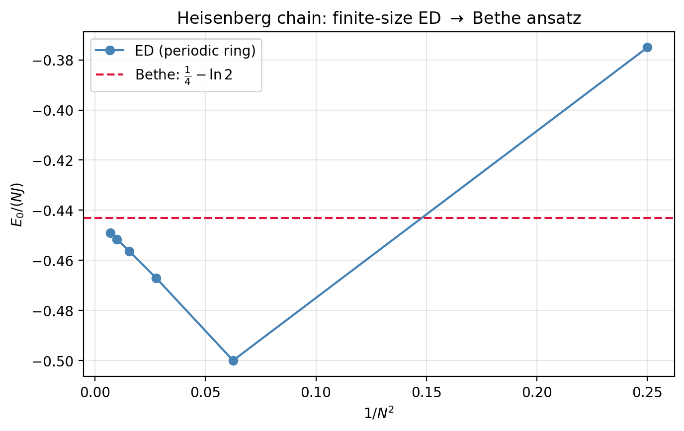
The spin chain is small enough to diagonalize directly: $N$ spins live in a $2^N$ space, and building ${\mathbf{S}}_i\cdot {\mathbf{S}}_j$ by Kronecker products then calling eigvalsh reaches $N=12$ (4096 states) on a laptop. The ground-state energies land exactly where they should:

Heisenberg spin-1/2 rings (J=1), ground state by ED vs known values:
  N= 2 ring:  E0 = -0.75000000    (exact -0.750000)
  N= 4 ring:  E0 = -2.00000000    (exact -2.000000)
  N= 6 ring:  E0 = -2.80277564    (exact -2.802776, diff 3e-11)
  N= 8 ring:  E0/N = -0.456387
  N=10 ring:  E0/N = -0.451545
  N=12 ring:  E0/N = -0.448949
  Bethe-ansatz thermodynamic limit:  e0/J = 1/4 - ln2 = -0.443147

Small even rings nail their exact values (the 4-site ring is $-2J$ to the bit; the 6-site ring is $-2.8028J$ to eleven digits), and the energy per site marches up toward Hans Bethe's 1931 thermodynamic-limit answer,

a number with no right to be that clean — a logarithm, from a spin chain, exact. Plotting against $1/N^2$ and extrapolating gets there from twelve spins. This is the same finite-size-scaling move as the Ising exponents, and it is honest about its one weakness: the 1D antiferromagnet is critical — gapless, correlations decaying as a power law, not exponentially — so the finite-size corrections fall off only algebraically and the extrapolation has to work for its digits.

What the ground state actually is

The classical picture — spins rigidly up, down, up, down — is not the ground state, and cannot be: ${\mathbf{S}}_i\cdot {\mathbf{S}}_j$ contains $S_i^x{S}_j^x+S_i^y{S}_j^y$ terms that flip neighboring pairs, so the true ground state is a massively entangled superposition of the Néel state and all its flipped descendants — a quantum antiferromagnet. Its excitations are not spin waves but fractionalized spinons carrying spin ½, and its entanglement entropy grows logarithmically with block size (central charge $c=1$), the fingerprint that puts it in the same universality class the DMRG page exploits: a 1D critical chain is exactly the regime matrix product states are built for, and DMRG computes this ground state to far larger $N$ than dense ED can reach. The area law and its logarithmic violation at criticality are the reason the method's bond dimension is the knob it is.

Extensions

• The $t/U$ corrections — go to fourth order and the effective model grows ring-exchange and further-neighbor terms; the Hubbard-to-Heisenberg map is the leading term of a controlled expansion, not an identity.
• The $t\text{–}J$ model — keep the superexchange but allow a few holes (dope away from half filling): the minimal model of a doped Mott insulator, and the leading candidate for cuprate superconductivity.
• Higher dimensions and DMRG — the 2D Heisenberg antiferromagnet does order (Néel, with reduced moment from quantum fluctuations); DMRG and quantum Monte Carlo on the square lattice pin the sublattice magnetization, while the triangular and kagome cases remain contested spin-liquid candidates.
• Frustration and the sign problem — frustrated magnets connect straight to why strongly correlated systems are computationally hard; a dedicated sign-problem page is the natural next stop.

Reproduce it

scripts/gen_hubbard.py builds the fermionic Hubbard Hamiltonian in a fixed particle-number sector (with Jordan–Wigner signs), diagonalizes it against the two-site closed form, and runs the Heisenberg ED and Bethe extrapolation above. Its one instructive bug is documented in the source: a two-site periodic ring has a single bond, but the naive loop $i\to (i+1)\mathrm{mod}L$ counts it twice, silently doubling $t$ and handing you a ground state that is exactly wrong by a factor tied to the geometry — caught only because the closed form was there to disagree with it.