Two-Site DMFT: The Mott Transition on a Laptop

The Mott transition page ends with a promise: the method that actually cracked the interaction-driven metal–insulator transition is dynamical mean-field theory. This page makes good on it in the smallest form that still works — Potthoff's two-site DMFT (2001), where the entire self-consistent machinery reduces to diagonalizing a 16-state impurity problem in a loop. It is a genuine DMFT calculation, it produces the Mott transition, and it lands the critical interaction within a few percent of the full numerical answer — on a laptop, in a screen of code. The reason it works is the one big idea worth carrying out of the whole subject: a lattice of interacting electrons can be replaced, exactly in infinite dimensions, by a single interacting site embedded in a self-consistent bath.

The idea: one site, and a bath that stands in for the rest

Static mean-field theory (Hartree–Fock) replaces the interaction each electron feels with an averaged number — and, as the Mott page showed, gets a paramagnetic Mott insulator qualitatively wrong, because a number cannot carry the frequency dependence a Mott gap lives in. DMFT keeps that frequency dependence. It freezes every site of the lattice but one, and replaces the frozen surroundings with a bath: a reservoir the one kept site exchanges electrons with, described by a hybridization function $\Delta (\omega )$ rather than a constant. The kept site plus its bath is a quantum impurity problem — an Anderson model — and it is solved exactly, correlations and all. The catch that closes the loop: the bath is not given, it is determined self-consistently by demanding that the impurity reproduce the lattice's own local Green's function. In the limit of infinite lattice coordination the self-energy becomes purely local and this replacement is exact — DMFT is the correct mean-field theory of a correlated lattice, the one that keeps $\omega$.

Two sites: truncate the bath to one orbital

The expensive part of DMFT is the impurity solver: the bath $\Delta (\omega )$ is a continuum, and reproducing it needs a powerful method (numerical renormalization group, continuous-time quantum Monte Carlo, or exact diagonalization with many bath orbitals). Potthoff's move is to keep only the leading physics of that bath by representing it with a single orbital. The impurity model becomes a two-site Anderson model — one correlated site, one bath site — with just two parameters, the bath energy ${\epsilon }_c$ and the hybridization $V$. Four spin-orbitals, sixteen states: exact diagonalization is instant.

At half filling, particle–hole symmetry does most of the bookkeeping for free — it pins the bath level to the Fermi energy (${\epsilon }_c=0$) and the impurity level to ${\epsilon }_d=-U/2$ — and the two-site self-consistency collapses to a single, transparent condition on the hybridization:

where $Z$ is the quasiparticle weight the impurity solution produces and $M_2$ is the second moment of the lattice density of states. The physics is legible right there: the hybridization the impurity sees is the bare bandwidth scale $M_2$ renormalized by the quasiparticle weight. As correlations kill $Z$, the bath decouples ($V\to 0$) and the site localizes. That is the Mott transition, waiting to fall out of a fixed-point iteration.

# Impurity: 2-site Anderson model (correlated site d + one bath orbital c),
# 4 spin-orbitals -> 16 states. c_op(p) = annihilation on orbital p (Jordan-Wigner);
# CD[p] = creation. anderson_H builds e_d n_d + e_c n_c + U n_up n_dn + V(d^dag c + h.c.).

def impurity_green(U, V, z):
    """Retarded impurity Green's function G_dd(z) at T=0, by the Lehmann sum."""
    H = anderson_H(U, V, ed=-U/2, ec=0.0)       # e_c=0, e_d=-U/2: half filling
    E, W = np.linalg.eigh(H)
    gs = W[:, 0];  dE = E - E[0]
    add = W.T @ (CD[0] @ gs)                     # <n| d^dag |0>  (add an electron)
    rem = W.T @ (C[0]  @ gs)                     # <n| d     |0>  (remove one)
    z = z[:, None]
    return (abs(add)**2/(z - dE)).sum(1) + (abs(rem)**2/(z + dE)).sum(1)

def quasiparticle_weight(U, V, w=1e-4):
    """Z = 1/(1 - dSigma/dw|_0) from the self-energy slope on the imaginary axis."""
    z = np.array([1j*w, 2j*w])
    Sigma = z + U/2 - V**2/z - 1/impurity_green(U, V, z)     # Sigma = G0^-1 - G^-1
    s = Sigma.imag / np.array([w, 2*w])
    return 1/(1 - (2*s[0] - s[1]))              # slope extrapolated to w -> 0

def solve_dmft(U, M2=0.25):                      # Bethe lattice: M2 = D^2/4, D=1
    """The DMFT loop: solve impurity -> get Z -> update bath V^2 = Z*M2 -> repeat."""
    Z = 1.0
    for _ in range(500):
        V = np.sqrt(Z * M2)
        Z = 0.5*Z + 0.5*quasiparticle_weight(U, V)
    return Z, np.sqrt(Z * M2)

The impurity Green's function is the exact $T=0$ Lehmann sum over the sixteen eigenstates: poles wherever adding or removing an electron connects the ground state to an excited one. The self-energy is $\Sigma =G_0^{-1}-G^{-1}$, its slope at zero frequency gives $Z$, and the loop feeds that $Z$ back into the bath. Run it:

Two-site DMFT, Bethe lattice, D=1  (M2 = D^2/4 = 0.25):

  impurity solver checks
    U=0:  Z = 1.0000000            self-energy vanishes (exact)
    sum rule   int A(w) dw = 0.99989   (per spin)
    U=0  G(z) vs analytic z/(z^2-V^2):  max |diff| = 3e-16

  self-consistent quasiparticle weight Z(U)
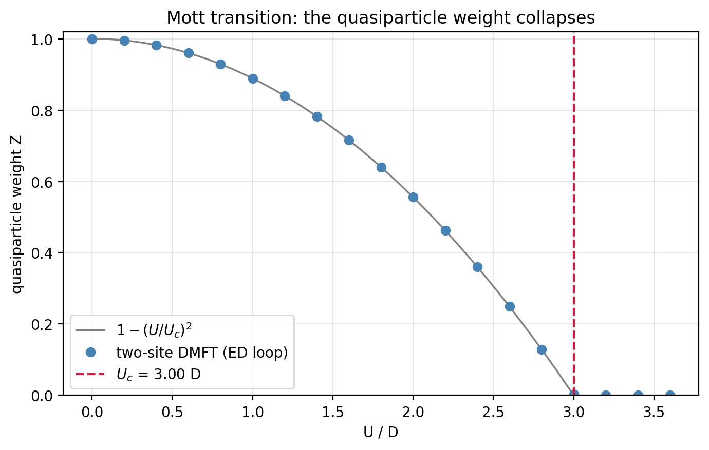
    U=1.0:  Z = 0.888889     ( = 1 - (1.0/3)^2 )
    U=2.0:  Z = 0.555556     ( = 1 - (2.0/3)^2 )
    U=2.4:  Z = 0.360000     ( = 1 - (2.4/3)^2 )
    U=2.8:  Z = 0.128889     ( = 1 - (2.8/3)^2 )
    U=3.0:  Z = 0.000000       Mott insulator

  Mott transition:  U_c = 3.000 D
  closed form Z = 1 - (U/U_c)^2 fits the ED loop to 2e-7
  full DMFT (NRG) reference:  U_c ~ 2.9 D   ->  two-site is within 4%

The quasiparticle weight collapses — exactly

The self-consistent loop does not just suggest a Mott transition — it reproduces a closed form. The quasiparticle weight follows the Brinkman–Rice law

and the exact-diagonalization loop lands on it to $2\times 10^{-7}$: $Z(U=1)=8/9$, $Z(U=2)=5/9$, $Z(U=2.4)=0.36$, straight down to zero at $U_c=3D$. The quasiparticle — the dressed, still-mobile electron of the correlated metal — grows heavier and heavier ($m^{\ast }/m=1/Z$) as $U$ rises, and at $U_c$ its weight vanishes: infinite effective mass, no more coherent charge carrier, an insulator. The number to be impressed by is $U_c=3D$. Full DMFT with an exact bath (numerical renormalization group) puts the transition at $U_c\approx 2.9D$ — so a single bath orbital, chosen by one moment condition, captures the Mott critical interaction to about four percent. That agreement is why the two-site scheme is a teaching tool and not just a toy.

The spectrum: a peak that dies, bands that survive

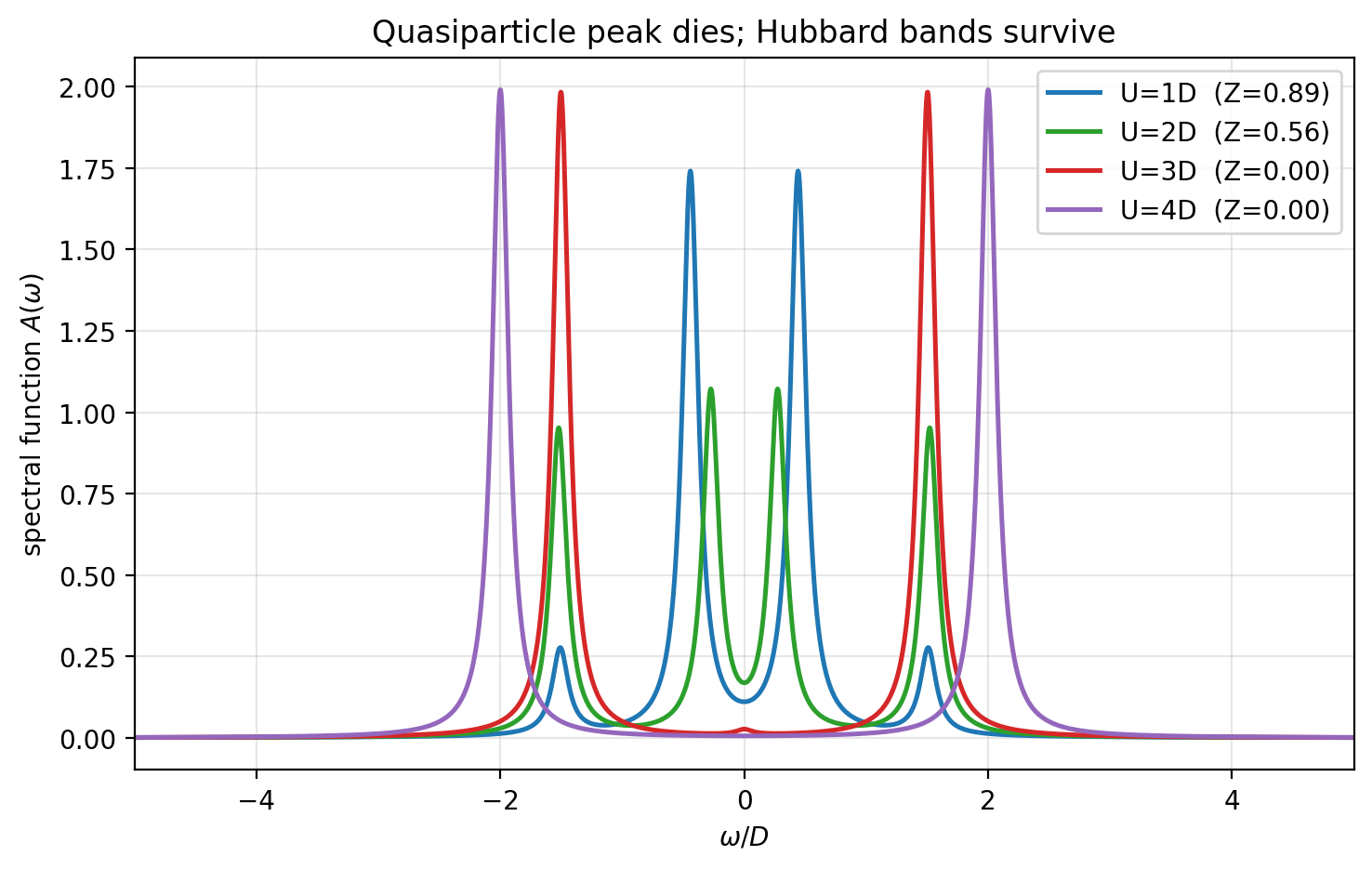
The single-particle spectral function $A(\omega )=-\frac{1}{\pi }\mathrm{Im}G(\omega )$ shows the transition as a transfer of spectral weight. At small $U$ there is a central quasiparticle peak at the Fermi level carrying weight $Z$ — the coherent metal. As $U$ grows, that peak loses weight to two Hubbard bands near $\pm U/2$, the incoherent excitations of adding an electron to an occupied site or removing one from an empty site. At $U_c$ the central peak is gone and only the split bands remain: the Mott gap. This three-feature structure — coherent peak between two Hubbard bands, the peak dying at the transition — is the signature DMFT picture, and here it emerges from sixteen states. (With only one bath orbital the bands are a few sharp poles rather than smooth continua; the shape is a cartoon, but the weight transfer and the gap are real.)

What one bath site can and cannot do

The trade-off is the point. Two-site DMFT gets the quasiparticle physics remarkably right — $U_c$, the mass divergence, the Brinkman–Rice law — because those are controlled by low-frequency moments, and a single bath orbital tuned to $M_2$ matches them. What it cannot do is the lineshape: the real Kondo resonance has a width and the real Hubbard bands are broad continua, and reproducing them needs a bath that can represent a continuous $\Delta (\omega )$ — many orbitals (exact-diagonalization DMFT), or a genuine continuum solver (NRG, CTQMC). Two-site DMFT is the $N_b=1$ member of a convergent family: add bath orbitals and the spectra fill in toward the exact answer, at the price of the exponential Hilbert space this page was built to avoid. Knowing which observables a cheap approximation nails and which it fakes is the whole skill.

Extensions

• More bath sites — exact-diagonalization DMFT with $N_b=4\text{–}8$ bath orbitals fits a continuous $\Delta (\omega )$ by least squares on the Matsubara axis; the spectra fill in and $U_c$ converges, at exponential cost in the impurity Hilbert space.
• Real impurity solvers — the numerical renormalization group (a Wilson-style logarithmic bath) and continuous-time QMC are the production solvers; two-site DMFT is the pedagogical $N_b=1$ limit of the same loop.
• Finite temperature and coexistence — away from $T=0$ the Mott transition is first-order, with a metal–insulator coexistence wedge ending at a critical point of the liquid–gas universality class — DMFT's signature phase diagram.
• Cluster DMFT and the 2D wall — DCA / cellular DMFT restore momentum dependence for the 2D Hubbard problem, and run into the sign problem in their solvers — the frontier this section keeps circling back to.

Reproduce it

scripts/gen_dmft.py builds the two-site Anderson impurity with Jordan–Wigner operators, solves it by dense diagonalization, computes the Lehmann Green's function and self-energy, and iterates $V^2=Z{M}_2$ to convergence. Three checks gate the physics before the loop is trusted: the impurity Green's function matches the analytic non-interacting form to $10^{-16}$, the spectral function integrates to one, and the $U=0$ self-energy vanishes so $Z=1$. Only then does the fixed point $Z=1-(U/3D{)}^2$ — and the Mott transition at $U_c=3D$ — mean anything.