The Mott Transition: When Repulsion Makes an Insulator

Band theory has a clean rule for who conducts: count the electrons per unit cell, fill the bands from the bottom, and if the last occupied band is only partly full you are a metal. A single half-filled band is the textbook metal. Yet a whole class of materials — transition-metal oxides like $\mathrm{NiO}$, the parent compounds of the high-temperature superconductors — have exactly that half-filled band and are stubbornly insulating, some of them deep purple and transparent where band theory promises a shiny conductor. Nevill Mott's answer (1949): the electrons don't conduct because they repel. Turn $U$ up in the Hubbard model and the same half-filled band that band theory calls a metal opens a gap and stops conducting — a metal–insulator transition driven by interaction alone, with no change in filling and no broken symmetry. This page measures that gap opening, straight out of exact diagonalization.

The gap you have to compute, not assume

Band theory's gap is a one-electron object — you read it off the dispersion. The Mott gap is not there in any band structure; it lives in the difference between many-body ground-state energies. The honest measure is the charge gap: the energy to add an electron plus the energy to remove one, i.e. how far the system resists a redistribution of charge.

def charge_gap(L, t, U):
    """The Mott gap at half filling: the cost to move charge, measured as
    E0(N+1) + E0(N-1) - 2 E0(N).  Each E0 is a Lanczos ground state
    (scipy eigsh) of the fermionic Hubbard H in a fixed (n_up, n_dn) sector."""
    n = L // 2                                  # half filling: N = L electrons
    E_N = hubbard_ground(L, t, U, n,   n)       # neutral
    E_p = hubbard_ground(L, t, U, n+1, n)       # add one electron
    E_m = hubbard_ground(L, t, U, n-1, n)       # remove one electron
    return E_p + E_m - 2*E_N

def double_occupancy(L, t, U):
    """<sum_i n_i,up n_i,dn> / L in the ground state — how often two electrons
    share a site. Band theory says 1/4; repulsion drives it to zero."""
    ...

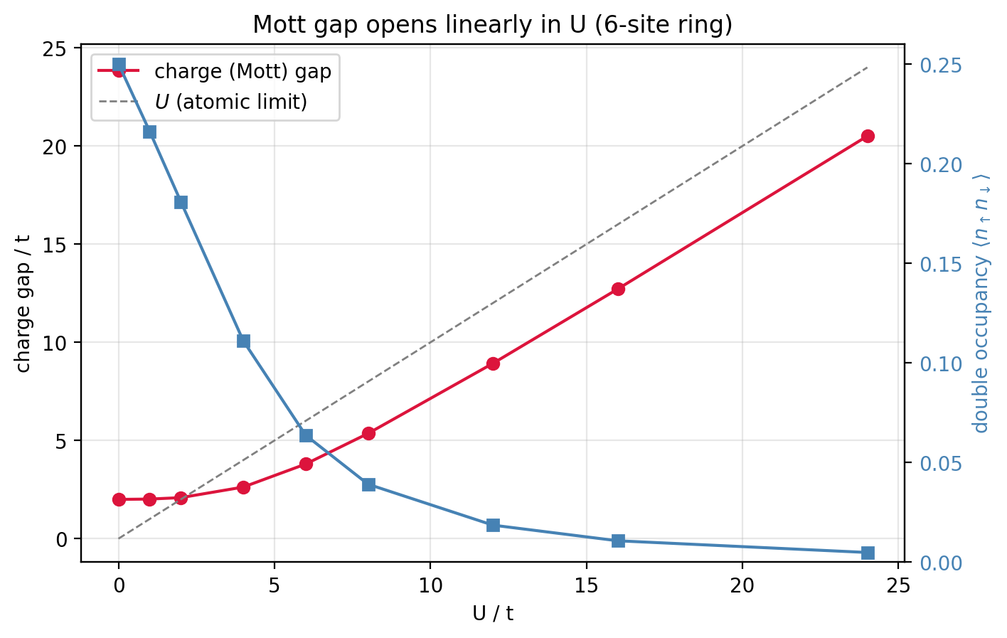
Each $E_0$ is a Lanczos ground state of the fermionic Hubbard Hamiltonian in its particle-number sector — the same engine the magnetism page uses. Run it across $U$ on a six-site ring:

Mott physics on a 6-site Hubbard ring (t=1):
  U      charge gap    double occupancy / site
  0.0     2.00000        0.25000     <- band-theory value 1/4
  1.0     2.01607        0.21613
  2.0     2.08869        0.18082
  4.0     2.62751        0.11107
  6.0     3.79938        0.06369
  8.0     5.35813        0.03911
 12.0     8.92593        0.01859
 16.0    12.71413        0.01075
 24.0    20.50399        0.00488
  large-U charge gap approaches U (atomic limit):  gap(24)/U = 0.854

Two curves tell the whole story. The charge gap starts near 2 at $U=0$ — that residual is finite size, the level spacing of a six-site ring, and it closes as the ring grows — then bends upward and becomes linear, tracking $U$ itself: at $U=24$ the gap is 20.5, i.e. $0.85U$, on its way to the atomic-limit value ${\Delta }_c\to U-W$ (the bare cost $U$ to make a double occupancy, minus the bandwidth $W$ the electron reclaims by delocalizing). That linear-in-$U$ gap is the Mott insulator: the more you repel, the harder it is to move charge.

The double occupancy is the mechanism in one number. At $U=0$ electrons are independent, so a site is up-occupied and down-occupied independently with probability $\frac{1}{2}$ each — $⟨n_{\uparrow }{n}_{\downarrow }⟩=\frac{1}{4}$ per site, exactly what the code reports. Crank $U$ up and it collapses: 0.25 → 0.11 → 0.039 → 0.005. The electrons are rearranging their wavefunction to avoid sharing sites, paying kinetic energy to dodge the repulsion. That avoidance is correlation — precisely the physics a single Hartree–Fock determinant cannot represent, which is why mean-field theory declares this system a metal and gets it qualitatively wrong.

Mott versus band: two ways to be an insulator

The distinction is the crux, and it is not pedantry. A band insulator — diamond, silicon — has an even number of electrons per cell filling bands completely; its gap is a one-electron property, robust and well described by DFT. A Mott insulator has an odd count, a half-filled band that band theory must call a metal, insulating only because of interaction. The tells are physical: a Mott insulator sits right at the edge of conducting, so pressure or doping can tip it metallic (or superconducting); and because the charges localize but their spins stay free, it is simultaneously a charge insulator and a quantum magnet — $J=4t^2/U$ is what those localized spins do next. A band insulator has no such spins and no such proximity to metallicity. Same word, opposite origin.

The frontier: DMFT and the wall at two dimensions

Exact diagonalization shows the gap opening but cannot follow the transition in the thermodynamic limit — the Hilbert space is $4^L$. The method that cracked the Mott transition is dynamical mean-field theory (Metzner–Vollhardt 1989; Georges–Kotliar 1992): map the entire lattice onto a single site exchanging electrons with a self-consistently determined bath — a quantum impurity problem — and solve that. The mapping becomes exact in infinite dimensions, and unlike static mean field it keeps the frequency dependence that a Mott gap lives in. DMFT delivered the picture textbooks now draw: a quasiparticle peak that narrows and dies as $U$ crosses a critical $U_c\sim W$, spectral weight bleeding into upper and lower Hubbard bands, and a first-order coexistence region at finite temperature. Its impurity solver is a Lanczos or continued-fraction spectral-function calculation — the same Krylov machinery the rest of this site leans on.

And the wall: DMFT is exact only in infinite dimensions. The physically urgent case — the two-dimensional Hubbard model, the minimal model of the cuprate superconductors — has no exact solution and no controlled numerical method that works at all fillings and temperatures. Quantum Monte Carlo, which would be the natural tool, runs into the fermion sign problem: away from half filling the sampling weights go negative and the statistical noise explodes exponentially. That the 2D Hubbard model — three parameters, written on one line — remains unsolved after forty years is the honest statement of where this frontier actually is.

Extensions

• The spectral function — resolve the gap in frequency: the Lanczos/continued-fraction spectral function of the Hubbard cluster shows the single quasiparticle band splitting into lower and upper Hubbard bands as $U$ grows — the Mott gap made visible in $A(\omega )$.
• Finite temperature and coexistence — the Mott transition is first-order at finite $T$, with a metal and insulator coexisting in a wedge of the phase diagram ending at a critical point — the same topology as liquid–gas, and DMFT's signature result.
• Doping the Mott insulator — the $t\text{–}J$ model and the 2D Hubbard model just off half filling: pseudogap, stripes, and $d$-wave superconductivity, the open problem this whole section circles.
• Why it's hard — the fermion sign problem is the reason the doped 2D case has no controlled solution; a dedicated page on it is the natural companion to this one.

Reproduce it

scripts/gen_hubbard.py computes every number here from the fermionic Hubbard Hamiltonian — the charge gap from three ground-state solves per $U$, the double occupancy from the ground-state vector. The engine is validated against the exact two-site closed form to machine precision before it is trusted on the six-site ring, which is the only reason the finite-size gap at $U=0$ can be read as geometry rather than a coding error.