Lanczos Iteration

Symmetric Lanczos is the Hermitian special case of Arnoldi iteration — and the simplification it brings is one of the cleanest payoffs in numerical linear algebra. When $A=A^T$, the upper-Hessenberg projection produced by Arnoldi collapses to a TRIDIAGONAL matrix, and the orthogonalisation against all previous Krylov vectors collapses to a THREE-TERM recursion against only the two most recent. Cost per step drops from $O(jn)$ to $O(n)$; storage drops from $O(mn)$ to $O(n)$. That collapse is what makes Lanczos the workhorse for extremal eigenvalues of symmetric sparse matrices and for evaluating $f(A)b$ on systems too large to factor.

Which collapse is which

Seeing Lanczos after Arnoldi feels like finishing a long calculation and then realizing the steps condense to three lines — and the danger of the condensed form is losing track of which simplification came from where. Here is the bookkeeping. Arnoldi builds $h_{jk}=q_j^{T}A{q}_k$ and must subtract every previous direction because any $h_{jk}$ might be nonzero. Now let $A=A^T$ and look at one entry: $h_{jk}=q_j^{T}A{q}_k=(A{q}_j{)}^T{q}_k$. But $A{q}_j$ lives in the span of $q_0,\dots ,q_{j+1}$ (that is what a Krylov process means), so for $k>j+1$ the entry is zero. The projection is therefore Hessenberg from Arnoldi and Hessenberg from symmetry — upper and lower at once — which is the definition of tridiagonal. That is collapse one.

Collapse two is the same zero pattern read row-wise instead of column-wise: in the orthogonalization sum $w=A{q}_k-{\sum }_j{h}_{jk}{q}_j$, every term with $j<k-1$ has just been shown to vanish, so the sum keeps exactly two terms — ${\alpha }_k{q}_k$ and ${\beta }_{k-1}{q}_{k-1}$ — and the loop over all previous vectors becomes the three-term recurrence. So there are not two separate miracles: the tridiagonal shape of $T$ and the shortness of the recurrence are one fact, seen once in the matrix and once in the loop. (And this is why floating point hurts Lanczos specifically: the recurrence trusts those provably-zero terms to stay zero, and round-off slowly makes them nonzero — the orthogonality decay the history section below is about.)

The history: a method that didn't work

Cornelius Lanczos published the algorithm in 1950 as a method for the FULL eigenvalue problem — tridiagonalize an $n\times n$ symmetric matrix by running the recurrence for all $n$ steps, then solve the resulting small tridiagonal eigenvalue problem. In exact arithmetic this is beautiful: $O(n)$ per step, constant memory, and the tridiagonal $T$ is similar to $A$ so its eigenvalues are exactly those of $A$.

In floating-point arithmetic it was a disaster. Round-off errors corrupt the orthogonality of the Lanczos vectors, and by the time the chain runs to length $n$ the resulting $T$ has nothing resembling the true eigenvalues — extra eigenvalues appear, real ones are mis-identified, multiplicities are wrong. By the late 1950s Householder tridiagonalization had been published, was numerically stable, and Lanczos was largely abandoned for full eigenproblems. The algorithm sat as a footnote for two decades.

The revival: stop running it to completion

Christopher Paige's 1971 PhD thesis (and a series of follow-up papers through 1976) showed something fundamental: the loss of orthogonality is not the disaster it looks like. The Ritz values produced by Lanczos still converge to the true eigenvalues of $A$, even as the basis vectors drift away from being orthogonal. The "ghost" eigenvalues that show up are re-discoveries of already-converged eigenvalues, produced when the drifted basis wanders back into the direction of a Ritz vector that already converged.

Paige's insight reframed the algorithm. Lanczos in its original form — run for $n$ steps to fully tridiagonalize $A$ — was abandoned for good. The MODERN use of Lanczos is iterative: run only $m\ll n$ steps, get approximations to the extremal eigenvalues of $A$. The loss of orthogonality never becomes catastrophic because you stop before it does, and convergence at the spectral edges is so fast that you usually need many fewer iterations than the matrix dimension to nail the dominant few eigenvalues to machine precision.

The variant zoo: 30 years of fixes

Even the iterative form needed a series of refinements. The succession of variants is the algorithm's actual development history:

• Plain Lanczos with no reorthogonalization (1950): cheap, ghost-prone. Usable if you post-process the eigenvalues to remove ghosts (Cullum-Willoughby, 1985).
• Full reorthogonalization (Wilkinson era, 1965): orthogonalize each new vector against all previous ones. Restores accuracy but destroys the algorithm's memory advantage — you're now running Arnoldi without admitting it.
• Selective reorthogonalization (Parlett-Scott, 1979): only reorth against the Ritz vectors that have converged, since those are the directions producing ghosts. Restores most of the memory advantage.
• Partial reorthogonalization (Simon, 1984): even cheaper — only reorth when the algorithm signals that orthogonality has eroded below a threshold.
• Implicit restarting (Sorensen, 1992): keep the Krylov subspace bounded by periodically filtering out unwanted eigenvalues using a polynomial shift. This is what ARPACK implements, and it's the algorithm most people actually run today.

The Padé connection

The Lanczos recurrence has the same shape as the recurrence for orthogonal polynomials, and the connection is not accidental: Lanczos is literally building the orthogonal polynomials with respect to the moment functional $⟨p(A)b,b⟩$. The convergents of the continued-fraction expansion of the resolvent $⟨(zI-A{)}^{-1}b,b⟩$ are exactly the $[m/m]$ Padé approximants to that resolvent, and the poles of those approximants are the Ritz values. So computing eigenvalues via Lanczos and approximating the resolvent via Padé are mathematically the same operation, viewed from two angles.

The Padé connection becomes practically essential for the non-symmetric case (see bi-orthogonal Lanczos). The biorthogonal recurrence can break down when the Padé table has a near-zero in the wrong place — the recurrence coefficients blow up. LOOK-AHEAD Lanczos (Freund, Gutknecht, Nachtigal, late 1980s) handles this by skipping over the bad entries in the Padé table, advancing by larger steps when necessary. The stable modern non-symmetric Lanczos algorithm is essentially a Padé-table navigator.

How the continued fraction falls out of the tridiagonal

The previous section asserted the equivalence — Lanczos coefficients are continued-fraction coefficients. Worth seeing exactly how. Three steps.

Step 1: Tridiagonal inverses are continued fractions

Take a symmetric tridiagonal $T$ with diagonal entries ${\alpha }_j$ and off-diagonals ${\beta }_j$. The top-left entry of $(T-\omega 1{)}^{-1}$ has a closed form:

Why? Cramer's rule. The $(0,0)$ entry of $T^{-1}$ is the $(0,0)$ cofactor divided by $\det T$. For a tridiagonal, both numerator and denominator are determinants of (smaller) tridiagonals related by a recursive formula — expand by the first row and you get a two-term recurrence in the dimension. That recurrence telescopes into the continued fraction above.

The chain by hand: a 3×3 you can follow on paper

Before any code, run the iteration yourself once. Take

Step 1. Apply the matrix: $A{v}_0$ is just the first column, $(2,1,1{)}^T$. The diagonal coefficient is its overlap with $v_0$: ${\alpha }_0=v_0^{T}A{v}_0=2$. Subtract that component: $(2,1,1{)}^T-2(1,0,0{)}^T=(0,1,1{)}^T$. What is left has length ${\beta }_0=\sqrt{2}$, and normalizing it gives the next basis vector $v_1=(0,1,1{)}^T/\sqrt{2}$.

Step 2. Apply the matrix again: $A{v}_1=(2,3,4{)}^T/\sqrt{2}$. Overlap with $v_1$: ${\alpha }_1=(0\cdot 2+1\cdot 3+1\cdot 4)/2=7/2$. Now subtract both the ${\alpha }_1{v}_1$ component and the ${\beta }_0{v}_0$ component — this double subtraction is the whole Lanczos three-term recurrence — and the residue works out to $(0,-1,1{)}^T/(2\sqrt{2})$, whose length is ${\beta }_1=1/2$. Normalize: $v_2=(0,-1,1{)}^T/\sqrt{2}$.

Step 3. $A{v}_2=(0,-3,4{)}^T/\sqrt{2}$, so ${\alpha }_2=(3+4)/2=7/2$ — and subtracting ${\alpha }_2{v}_2+{\beta }_1{v}_1$ leaves exactly zero: three orthonormal vectors span all of ${\mathbb{R}}^3$, so the chain must terminate. The full output of the iteration is

Now the continued fraction, by hand, at $\omega =5$. Depth 1 keeps only ${\alpha }_0$: $1/(5-2)=1/3$. Depth 2 hangs the first rung: $1/(3-2/(5-\frac{7}{2}))=1/(3-\frac{4}{3})=3/5$. Depth 3 nests the last rung, working from the bottom up: the innermost piece is $(1/2{)}^2/(5-\frac{7}{2})=\frac{1}{6}$; that makes the middle denominator $5-\frac{7}{2}-\frac{1}{6}=\frac{4}{3}$; so the first rung contributes ${\beta }_0^2/\frac{4}{3}=2\cdot \frac{3}{4}=\frac{3}{2}$, and the top level reads $1/(3-\frac{3}{2})=2/3$. Check it against the matrix directly: $\det (5I-A)=3$, the $(0,0)$ minor is $2$, so $[(5I-A{)}^{-1}{]}_{00}=2/3$ — exact agreement, and exactly at depth 3, because a 3×3 chain has only three rungs to give. The truncation sequence $1/3\to 3/5\to 2/3$ is the method compressed into three fractions.

Be clear about what this toy does and does not show. It shows the mechanics faithfully: the three-term recurrence, where each $\alpha$ and $\beta$ comes from, why the chain terminates, how the fraction telescopes. But a 3×3 is a special case in the way that matters most: three Lanczos steps span the entire space, so nothing is being compressed — the exactness at depth 3 is guaranteed for any $n\times n$ matrix at depth $n$, and is precisely the property you can never afford to use. The method exists for the regime $m\ll n$: you take a handful of steps, stop, and the truncated fraction is already close — a race between fraction depth and accuracy that a 3×3 cannot even exhibit. (Floating point adds a second thing the toy hides: over many steps the $v_j$ drift out of orthogonality and real implementations must reorthogonalize.) The 8×8 below shows the genuine situation — five steps against an eight-dimensional space — and the production habitat is bigger still: the shell-model page runs this same recurrence at dimension 28,503.

Watch it converge, with real numbers

Here is the whole mechanism on an actual matrix — an 8×8 random symmetric A (seed 3, spectrum spanning −4.10 to 3.94), start vector e₀, evaluated at ω = 5, safely outside the spectrum. Five Lanczos steps produce these coefficients:

import numpy as np
np.random.seed(3)
M = np.random.randn(8, 8); A = (M + M.T) / 2
q = np.zeros(8); q[0] = 1.0            # start vector e0
V, alphas, betas, qm, beta = [q], [], [], np.zeros(8), 0.0
for k in range(5):
    w = A @ q - beta * qm
    a = q @ w; alphas.append(a); w -= a * q
    for u in V: w -= (u @ w) * u        # full reorthogonalization
    beta = np.linalg.norm(w)
    if k < 4: betas.append(beta)
    qm, q = q, w / beta; V.append(q)
# alphas: +1.7886 -0.4701 -0.8513 +1.2597 -1.1675
# betas :  2.2584  2.6923  1.7877  0.7346

Now build the continued fraction one level at a time and compare against the exact answer, [(5·I − A)⁻¹]₀₀ = 0.51535311, computed by direct inversion. Depth 1 uses only α₀: 1/(5 − 1.7886) = 0.3114. Depth 2 folds in the first off-diagonal: 1/(5 − 1.7886 − 2.2584²/(5 + 0.4701)) = 0.4388. Each level after that nests one more β²/(ω − α) rung at the bottom:

depth 1: 0.31139343   error 2.0e-01
depth 2: 0.43879403   error 7.7e-02
depth 3: 0.49850313   error 1.7e-02
depth 4: 0.51480508   error 5.5e-04
depth 5: 0.51530549   error 4.8e-05
exact  : 0.51535311

Five matrix–vector products pin an entry of the inverse to five decimal places — no inverse ever formed, no linear system solved. Each additional (α, β) pair buys roughly another digit, because each level of the fraction is exactly one more moment of A seen from the start vector. This is the trade the whole Krylov business runs on. Same trick that gives you the continued-fraction expansion of irrational numbers from their Euclidean-algorithm remainders, applied here to a polynomial of $\omega$.

Step 2: Lanczos delivers exactly such a tridiagonal

That's the entire point of the algorithm. Given an operator $A$ and a starting vector $v_0$, Lanczos builds an orthonormal Krylov basis $\{v_0,v_1,v_2,\dots \}$ in which the matrix of $A$ is tridiagonal. The diagonal entries are ${\alpha }_j=⟨v_j|A|v_j⟩$, the off-diagonals ${\beta }_j=⟨v_{j+1}|A|v_j⟩$. These are the Lanczos coefficients — and they are also the entries of the tridiagonal $T$ you'd plug into the continued fraction in step 1.

Step 3: The resolvent matrix element projects onto the tridiagonal's inverse

In the Lanczos basis, the matrix element $⟨v_0|(A-\omega {)}^{-1}|v_0⟩$ becomes, after projecting onto the Krylov subspace and inverting there, the $(0,0)$ entry of $(T-\omega 1{)}^{-1}$. In the full-dimensional limit (chain runs to completion) the two are equal exactly; in finite-dimensional truncations they agree to leading orders in the Padé sense. Combining with step 1:

The resolvent matrix element you want is a continued fraction in the Lanczos coefficients. Not because anyone designed it that way — because that's what tridiagonal inverses ARE and Lanczos produces a tridiagonal. The continued fraction isn't a separate trick stapled onto the algorithm; it's Cramer's rule reading off the inverse of what Lanczos already built.

The deeper structure

Continued fractions are the natural form for the STIELTJES TRANSFORM of a positive measure $d\mu$ on the real line — the integral $S(\omega )=\int d\mu (\lambda )/(\omega -\lambda )$. Lanczos coefficients ${\alpha }_j,{\beta }_j$ are the three-term-recurrence coefficients of the orthogonal polynomials with respect to the spectral measure of $A$. So "Lanczos gives a continued fraction for $⟨v_0|(A-\omega {)}^{-1}|v_0⟩$" and "the Stieltjes transform of a positive measure is the continued fraction whose coefficients are the recurrence coefficients of its orthogonal polynomials" are the same statement. This is the HAMBURGER MOMENT PROBLEM in disguise. Akhiezer's classical monograph and Stahl-Totik's General Orthogonal Polynomials are where to chase the full theory.

Practical implication: any time you need a quantity of the form "matrix element of a resolvent" — optical absorption spectra in TDDFT (see Liouville-Lanczos), Green's-function densities of states in solid-state physics, impurity-spectrum functions in DMFT — the right tool is Lanczos plus the continued fraction. The two are pieces of one machine.

A direct numerical check

Worth running the comparison yourself. Build a random 40×40 symmetric matrix, pick a unit vector, compute $⟨v_0|(A-\omega 1{)}^{-1}|v_0⟩$ by direct solve, then again by Lanczos plus continued fraction. The two answers should agree to machine precision when the chain runs to full dimension $N$, and the truncated chain should converge to the direct answer as the chain grows.

# Lanczos <-> continued-fraction correspondence: a verification.
# For a random 40x40 symmetric A and unit vector v0, compute
# G(omega) = <v0 | (A - omega I)^-1 | v0> two ways:
#   (1) Direct: solve (A - omega I) x = v0, return v0 @ x.
#   (2) Via Lanczos: build alphas, betas, evaluate the continued fraction.
# They should agree to machine precision when the chain runs to full N.

import numpy as np

rng = np.random.default_rng(42)
N = 40
H = rng.standard_normal((N, N))
A = (H + H.T) / 2.0
v0 = rng.standard_normal(N); v0 /= np.linalg.norm(v0)

def lanczos(A, v0, n_iter):
    """Symmetric Lanczos with full reorthogonalization."""
    alphas, betas, Q = [], [], [v0.copy()]
    q_prev = np.zeros_like(v0); q = v0.copy(); beta_prev = 0.0
    for j in range(n_iter):
        w = A @ q
        alpha = q @ w
        w = w - alpha * q - beta_prev * q_prev
        for qk in Q[:-1]:                       # full reorth
            w -= (qk @ w) * qk
        beta = np.linalg.norm(w)
        alphas.append(alpha)
        if beta < 1e-14: break
        if j < n_iter - 1:
            betas.append(beta)
            q_prev = q; q = w / beta
            Q.append(q.copy())
    return np.array(alphas), np.array(betas)

def cf_eval(alphas, betas, omega):
    """Evaluate the continued fraction bottom-up."""
    z = alphas[-1] - omega
    for j in range(len(alphas) - 2, -1, -1):
        z = (alphas[j] - omega) - betas[j]**2 / z
    return 1.0 / z

def resolvent_direct(A, v0, omega):
    x = np.linalg.solve(A - omega * np.eye(A.shape[0]), v0)
    return v0 @ x

alphas, betas = lanczos(A, v0, N)
eigvals = np.linalg.eigvalsh(A)

# Frequency sweep, offset eta above the real axis
def err_at_eta(eta, n):
    om = np.linspace(eigvals.min()-1, eigvals.max()+1, 25) + 1j*eta
    G_d = np.array([resolvent_direct(A, v0, w) for w in om])
    a, b = alphas[:n], betas[:n-1]
    G_n = np.array([cf_eval(a, b, w) for w in om])
    return np.max(np.abs(G_d - G_n))

print(f"Full chain (n={N}): max error = {err_at_eta(0.5, N):.3e}")
print(f"{'chain':>6}   eta=2.0           eta=1.0           eta=0.5")
for n in [4, 8, 12, 16, 20, 24, 28, 32, 36, 40]:
    print(f"{n:>6}   {err_at_eta(2.0, n):>15.3e}   "
          f"{err_at_eta(1.0, n):>15.3e}   {err_at_eta(0.5, n):>15.3e}")

Run it:

Full chain (n=40): max error = 3.886e-16
 chain   eta=2.0           eta=1.0           eta=0.5
     4         4.131e-02         1.803e-01         4.880e-01
     8         4.223e-03         5.098e-02         2.240e-01
    12         6.467e-04         2.146e-02         1.386e-01
    16         6.055e-05         5.690e-03         6.177e-02
    20         3.481e-06         1.036e-03         2.216e-02
    24         1.978e-07         2.373e-04         1.109e-02
    28         1.353e-08         5.361e-05         5.467e-03
    32         3.865e-10         1.074e-05         2.360e-03
    36         1.246e-12         3.403e-07         2.624e-04
    40         1.367e-16         3.297e-16         3.886e-16

Two things to read off. First, the full-chain agreement is at $10^{-16}$ — the correspondence isn't approximate, it's exact (up to floating-point noise). Second, the convergence under truncation depends sensitively on how close $\omega$ is to the spectrum: far away ($\eta =2.0$) you get clean geometric-Padé decay, gaining about an order of magnitude per two Lanczos iterations. Right next to the spectrum ($\eta =0.5$) the continued fraction has to "see" each eigenvalue before it can reproduce the nearby resolvent — so convergence is slow until the chain captures essentially the whole spectrum, then collapses to machine precision in the last few iterations.

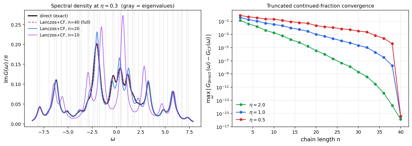
The plot says the same thing visually. Left panel: the spectral density $\mathrm{Im}G(\omega )/\pi$ at $\eta =0.3$. Black is the direct calculation; the red dashed line behind it is the full-chain Lanczos+CF result — they overlap. The $n=20$ truncation (blue) tracks the direct answer over most of the spectrum but loses fine detail; the $n=10$ truncation (purple) only resolves the gross structure. Right panel: error vs chain length at three $\eta$s, with the geometric decay at large $\eta$ and the slow-then-sudden collapse at small $\eta$ visible directly.

Why three terms

Build an orthonormal basis $\{q_0,q_1,\dots \}$ of the Krylov subspace ${\mathcal{K}}_m(A,b)$. By orthogonality, the new vector $A{q}_j$ expands as $A{q}_j={\sum }_{i=0}^{j+1}{h}_{ij}{q}_i$ with $h_{ij}=⟨q_i|A{q}_j⟩$. For Hermitian $A$ we can use $⟨q_i|A{q}_j⟩=⟨A{q}_i|q_j⟩$. Both $q_i$ and $A{q}_i$ live in the Krylov subspace of dimension $i+2$, so the inner product vanishes whenever $j>i+1$. Combining with the standard Arnoldi argument ($h_{ij}=0$ for $i>j+1$) gives:

So only THREE coefficients per column are non-zero: the diagonal ${\alpha }_j=⟨q_j|A{q}_j⟩$ and the two off-diagonal entries ${\beta }_j=⟨q_{j+1}|A{q}_j⟩=⟨q_j|A{q}_{j+1}⟩$ (the latter two equal by symmetry). The matrix $T=Q^{T}AQ$ is tridiagonal:

And the recursion that builds the basis is:

Rearranging, ${\beta }_j{q}_{j+1}=A{q}_j-{\alpha }_j{q}_j-{\beta }_{j-1}{q}_{j-1}$. Computing the next basis vector requires only the current and previous one — never the older ones. That's the famous "three-term recursion" and the reason Lanczos's memory footprint is constant in the chain length.

The algorithm

# Symmetric Lanczos — the Hermitian special case of Arnoldi.
# Three-term recursion in place of full Gram-Schmidt:
#    A q_j = beta_{j-1} q_{j-1} + alpha_j q_j + beta_j q_{j+1}
# Output: Q (n x m) with orthonormal columns, and tridiag T with diagonal
# alpha and off-diagonal beta:
#    Q^T A Q = T,  with T = tridiag(beta, alpha, beta).
# Crucially, only THREE vectors (q_prev, q, q_next) need to be in memory
# at once — independent of how long the chain runs.

import numpy as np

def lanczos(A, b, m):
    n = A.shape[0]
    Q = np.zeros((n, m))
    alphas = np.zeros(m)
    betas  = np.zeros(m - 1)
    q = b / np.linalg.norm(b)
    q_prev = np.zeros(n)
    beta = 0.0
    for j in range(m):
        Q[:, j] = q
        v = A @ q - beta * q_prev          # subtract the j-1 direction
        alpha = q @ v                      # diagonal entry
        alphas[j] = alpha
        v = v - alpha * q                  # subtract the j direction
        if j < m - 1:
            beta = np.linalg.norm(v)
            betas[j] = beta
            if beta < 1e-12:
                return Q[:, :j+1], alphas[:j+1], betas[:j]
            q_prev = q
            q = v / beta
    return Q, alphas, betas

# ─── Validation on a symmetric, well-conditioned matrix ─────────────────
np.random.seed(0)
n, m = 40, 15
A = np.random.randn(n, n)
A = (A + A.T) / 2 + n * np.eye(n)        # symmetric, SPD by construction
b = np.random.randn(n)

Q, alphas, betas = lanczos(A, b, m)
T = np.diag(alphas) + np.diag(betas, 1) + np.diag(betas, -1)

print(f"max |Q^T Q - I|   = {np.max(np.abs(Q.T @ Q - np.eye(m))):.2e}")
print(f"max |Q^T A Q - T| = {np.max(np.abs(Q.T @ A @ Q - T)):.2e}")

ritz = np.sort(np.linalg.eigvalsh(T))
true = np.sort(np.linalg.eigvalsh(A))
print(f"Smallest:  Ritz {ritz[0]:.5f}    true {true[0]:.5f}    diff {abs(ritz[0]-true[0]):.2e}")
print(f"Largest:   Ritz {ritz[-1]:.5f}    true {true[-1]:.5f}    diff {abs(ritz[-1]-true[-1]):.2e}")

# Demonstration: loss of orthogonality at long chain length
Q_long, _, _ = lanczos(A, b, m=35)
print(f"After m=35 iters: max |Q^T Q - I| = {np.max(np.abs(Q_long.T @ Q_long - np.eye(35))):.2e}")

Output on a 40×40 symmetric positive-definite matrix with $m=15$:

max |Q^T Q - I|   = 2.46e-13
max |Q^T A Q - T| = 8.87e-12
Smallest:  Ritz 30.88945    true 30.88945    diff 7.68e-07
Largest:   Ritz 48.20060    true 48.20061    diff 1.28e-05
After m=35 iters: max |Q^T Q - I| = 4.10e-03

Three things to read off. (1) Orthogonality holds to $\sim 10^{-13}$ and the tridiagonal relation $Q^{T}AQ=T$ to $\sim 10^{-12}$ — both at the level of typical accumulated round-off. (2) The smallest and largest Ritz values (eigenvalues of $T$) match the true extremal eigenvalues of $A$ to many decimal places after just 15 iterations on a 40-dim problem. This rapid convergence at the SPECTRAL EDGES is the central practical strength of Lanczos for symmetric eigenproblems. (3) The third number reveals the famous gotcha.

Which eigenvalues converge first?

Lanczos doesn't give you arbitrary eigenvalues of $A$; it gives you the EXTREMAL ones — the largest and smallest — and then works inward. After $m$ iterations the Ritz values approximate the true eigenvalues with a strong outside-in bias: the very largest and very smallest Ritz values are accurate first, then the second-largest and second-smallest, and so on. Interior eigenvalues (near the middle of the spectrum) converge slowly or, in practice, not at all without help.

The convergence rate is set by the SPECTRAL GAP. If the largest eigenvalue ${\lambda }_1$ is well-separated from ${\lambda }_2$, the corresponding Ritz value converges geometrically with rate determined by $({\lambda }_1-{\lambda }_2)/({\lambda }_1-{\lambda }_n)$. A well-separated extremal eigenvalue can be nailed to machine precision in tens of iterations even on million-dimensional matrices. A clustered or interior eigenvalue can require thousands.

This bias is why Lanczos is the natural tool for "ground state" problems — lowest eigenvalue of a Hamiltonian, second-smallest eigenvalue of a graph Laplacian (the Fiedler value), top few principal components — and why it's the wrong tool for "I need the 500th eigenvalue specifically." For interior eigenvalues you reach for shift-invert (apply Lanczos to $(A-\sigma I{)}^{-1}$ instead of $A$, which moves the eigenvalue closest to $\sigma$ to the extremum) or for polynomial-filtered variants like the Davidson method.

Loss of orthogonality

Extending the chain to 35 iterations, the residual orthogonality error climbs to $\sim 10^{-3}$ — eleven orders of magnitude worse than at iteration 15. This is not a bug in the algorithm; it is intrinsic to the no-re-orthogonalisation Lanczos recursion in finite precision. As Ritz values converge to true eigenvalues, the directions they correspond to get amplified in the basis. Tiny round-off errors that point along already-converged directions are not subtracted by the three-term recursion (since those directions only show up in $q_{j-1},q_j$), so they accumulate.

The effect was identified by Paige (1971-1976) and analyzed in detail by Cullum and Willoughby. The pathology in the eigenvalue problem is the production of "GHOST" Ritz values: spurious duplicate eigenvalues that appear when a converged Ritz value is re-discovered along a drifted basis vector. Distinguishing ghosts from genuine multiplicities requires either re-orthogonalisation (expensive, restores Arnoldi cost) or post-hoc filtering (Cullum-Willoughby ghost test). For most extremal-eigenvalue applications a small partial re-orthogonalisation against converged Ritz vectors is enough.

For the resolvent / continued-fraction applications (see bi-orthogonal Lanczos and Liouville-Lanczos), loss of orthogonality is essentially benign: ghost eigenvalues contribute zero residue to the matrix element you actually care about. The chain coefficients are still the continued-fraction coefficients of the true resolvent.

What it's used for

• Extremal eigenvalues of symmetric sparse matrices. Ground states of large Hamiltonians, lowest-frequency vibrational modes, second-smallest eigenvalue of a graph Laplacian. After $m\ll n$ iterations the smallest few Ritz values are converged to machine precision in the well-separated cases.
• Matrix functions $f(A)b$. The Lanczos approximation is $f(A)b\approx \Vert b\Vert Q_{m}f(T_m)e_1$. Useful for $\exp (A)b$ in quantum time-propagation, $A^{-1/2}b$ in Gaussian sampling, and anything Lanczos-quadrature.
• Tridiagonalisation as a precursor. Many algorithms (e.g. for spectral density estimation) want a tridiagonal that can be analyzed downstream.
• The conjugate-gradient connection. CG for solving $Ax=b$ is mathematically Lanczos on $A$ with a clever reorganisation of the iterates so the basis is never stored explicitly. The CG residuals are scalar multiples of the Lanczos basis vectors.

Related methods

• Power iteration — keeps only the latest direction; converges to the dominant eigenvector. Lanczos keeps all of them and gets many extremal eigenvalues at once.
• Arnoldi iteration — the non-symmetric parent. Without $A=A^T$, the tridiagonal collapse fails and you're stuck with full Gram-Schmidt at every step.
• Bi-orthogonal Lanczos — recovers tridiagonal structure for non-Hermitian $A$ by maintaining two Krylov sequences. The Liouville-Lanczos TDDFT method uses this generalization.
• Davidson method — preconditioned Lanczos-flavoured iteration tuned for the eigenvalue problems in electronic-structure theory.
• Conjugate gradient — Lanczos's reorganisation for solving $Ax=b$ when $A$ is SPD.