Project: Critical Exponents from Finite-Size Scaling

Four exact exponents extracted from lattices no bigger than 128×128 — and the reason a 2.3% "miss" on the GPU Ising page was never an error. Stack: Python · NumPy · numba.

The GPU Ising project located the susceptibility peak of a 64×64 lattice at $T=2.323$ and noted, almost apologetically, that Onsager says 2.269. Nothing was wrong. A finite lattice has no phase transition at all — the peak must sit off the true $T_c$, shifted by an amount that shrinks as a power of $L$. Finite-size scaling is the discipline that turns that annoyance inside out: instead of fighting the drift, you measure how observables drift with L, and the drift rates are the critical exponents. This page runs the full pipeline on the 2D Ising model, where every answer is known exactly — $T_c=2/\ln (1+\sqrt{2})$, $\beta =1/8$, $\gamma =7/4$, $\nu =1$ — so every step of the method is checkable to the digit.

First problem: Metropolis dies exactly where you need it

At $T_c$ the correlation length wants to be infinite, and single-spin flips move information one site at a time. The autocorrelation time of Metropolis grows as $\tau \sim L^z$ with $z=2.1667(5)$ (Nightingale & Blöte, PRB 62, 1089 (2000)) — double the lattice, pay four times the sweeps per independent sample, on top of the four-fold cost per sweep. Wolff's cluster algorithm (Wolff, PRL 62, 361 (1989)) deletes the problem: grow a cluster of aligned spins by adding each aligned neighbor with probability $p=1-e^{-2\beta }$, then flip the whole thing. That particular $p$ is the unique choice that makes the move rejection-free while preserving detailed balance, and it drops $z$ to nearly zero.

@njit(cache=True)
def wolff_run(spins, nbr, T, n_steps, seed):
    """n_steps Wolff cluster updates; returns per-step m and cluster sizes."""
    np.random.seed(seed)
    N = spins.size
    p_add = 1.0 - np.exp(-2.0 / T)     # Wolff's magic bond probability
    stack = np.empty(N, dtype=np.int64)
    mag = spins.sum()
    for step in range(n_steps):
        seed_site = np.random.randint(N)
        s0 = spins[seed_site]
        spins[seed_site] = -s0          # flip as you go: no visited[] array
        stack[0] = seed_site
        top = 1
        csize = 1
        while top > 0:                  # grow the cluster depth-first
            top -= 1
            site = stack[top]
            for k in range(4):
                j = nbr[site, k]
                if spins[j] == s0 and np.random.random() < p_add:
                    spins[j] = -s0
                    stack[top] = j
                    top += 1
                    csize += 1
        mag -= 2 * s0 * csize           # the whole cluster flipped at once

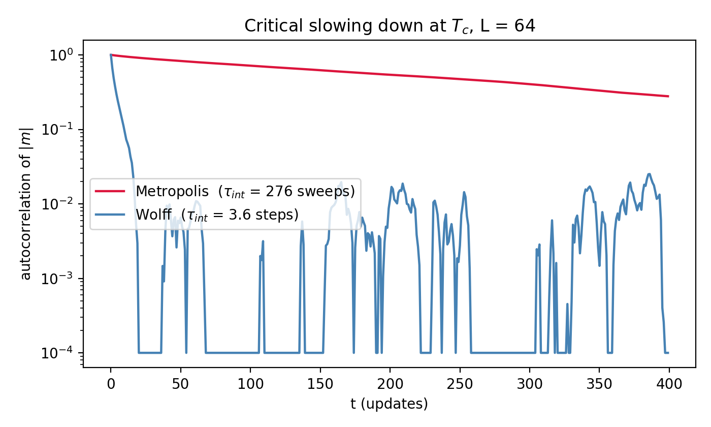
Measured at $T_c$ on a 64×64 lattice, with the integrated autocorrelation time computed by Sokal's self-consistent window:

def tau_int(series, c=6.0):
    """Integrated autocorrelation time with the Sokal self-consistent window."""
    x = series - series.mean()
    n = len(x)
    acf = np.correlate(x, x, mode='full')[n - 1:] / (np.arange(n, 0, -1) * x.var())
    tau = 0.5
    for W in range(1, n // 3):
        tau = 0.5 + acf[1:W + 1].sum()
        if W >= c * tau:               # stop summing when the window
            break                      # exceeds c times the answer
    return tau

At Tc, L=64:  tau_int(|m|)  Metropolis = 275.8 sweeps
              tau_int(|m|)  Wolff      = 3.56 steps
              mean cluster = 1585 spins = 0.387 sweeps of work
              work-normalized Wolff tau = 1.378 sweep-equivalents
              speedup at L=64 ~ 200x

One Wolff step costs less than a full sweep of work (the mean cluster is a fraction of the lattice), and its samples decorrelate in a couple of steps. Everything below uses Wolff; the same statistics with Metropolis would multiply the compute by two orders of magnitude at the largest $L$ — and the gap widens as $L^z$.

The Binder cumulant: a dimensionless quantity crosses at one point

The fourth-order cumulant of the magnetization (Binder, Z. Phys. B 43, 119 (1981)),

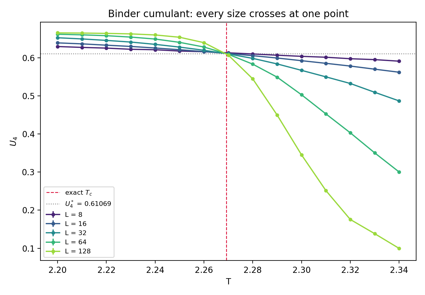
is built to be dimensionless: near criticality it depends on $T$ and $L$ only through the single combination $(T-T_c)L^{1/\nu }$. At $T=T_c$ that combination is zero for every $L$ — so the $U_4(T)$ curves of all lattice sizes pass through one point. Plot five sizes, find the crossing, and you have located an infinite-volume phase transition using boxes that fit in a laptop's cache:

U4 crossing L=8/16:   T = 2.26358   U4 = 0.61448
U4 crossing L=16/32:  T = 2.26657   U4 = 0.61289
U4 crossing L=32/64:  T = 2.26476   U4 = 0.61477
U4 crossing L=64/128: T = 2.25590   U4 = 0.63188

Tc estimate  = 2.26241   (exact 2.26919, error 0.299%)
U4* estimate = 0.61985   (Kamieniarz-Blote 0.61069)

The crossing value itself is a universal number — every system in the 2D Ising universality class shares it. The benchmark is $U_4^{\ast }=0.61069$ (Kamieniarz & Blöte, J. Phys. A 26, 201 (1993)), with the caveat that it depends on boundary conditions and aspect ratio, so it identifies your setup as much as your model.

Look at the table before moving on: the three mid-size crossings cluster within 0.25% of the exact answer, and then the 64/128 crossing sits visibly low. Diagnosis, not hand-waving: the crossings are located by intersecting cubic fits of $U_4(T)$ over the whole temperature window, and at $L=128$ the true curve has become so steep (its slope grows as $L^{1/\nu }$) that a cubic can no longer follow it — the interpolant, not the physics, moves the crossing. The tell is that tripling the sample count at $L=128$ moved this crossing by 0.00008: statistics-immune errors are systematic errors. The same underfit derivative is why the $\nu$ estimate below is the weakest of the four numbers. A narrower fit window around the crossing is the standard cure — left as the first exercise for anyone reproducing this.

Two exponents from five lattice sizes

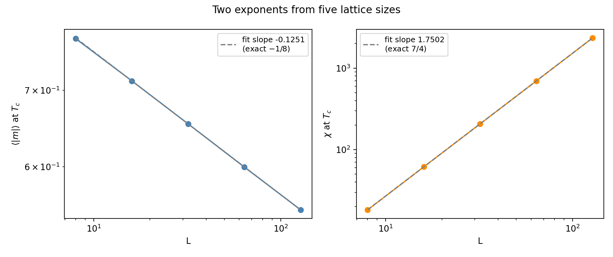
Sit exactly at $T_c$ (we know it; that is the luxury of 2D) and watch observables change with $L$ alone. Scale invariance forces pure power laws: $⟨|m|⟩\sim L^{-\beta /\nu }$ and $\chi \sim L^{\gamma /\nu }$. On a log-log plot the exponents are slopes:

beta/nu  = 0.1251   (exact 0.1250, error 0.1%)
gamma/nu = 1.7502   (exact 1.7500, error 0.0%)
1/nu     = 1.1075  ->  nu = 0.9030   (exact 1.0, error 9.7%)

Data collapse — and what failure looks like

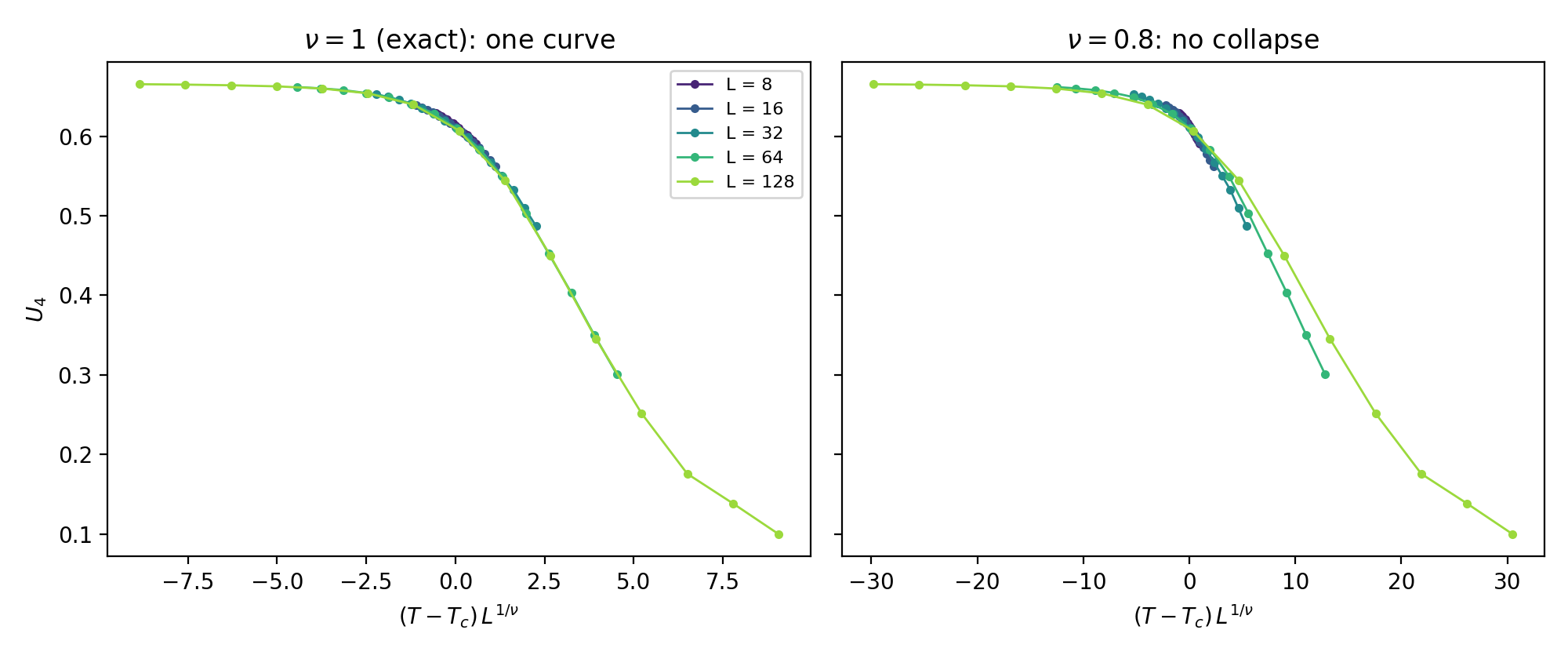
The scaling hypothesis makes one more prediction, stronger than any single exponent: plotted against $(T-T_c)L^{1/\nu }$, the $U_4$ data for all sizes and all temperatures must fall on a single curve. With the exact $\nu =1$ they do. And the test has teeth — feed it a wrong exponent and the curves fan apart:

This is the falsifiability picture. Data collapse is not a fit that always "sort of works" — a 20% error in $\nu$ is visible from across the room.

Why this works at L ≤ 128 — and why 3D took thirty years

Every scaling law above has corrections of order $L^{-\omega }$. The 2D Ising model is charmed: $\omega \approx 2$, so at $L=64$ the corrections sit at the 10⁻⁴ level and small lattices tell the truth. In 3D, $\omega =0.832(6)$ — corrections die so slowly that state-of-the-art Monte Carlo needed lattices up to 1024³ and careful correction-to-scaling fits to reach $K_c=0.221654626(5)$ (Ferrenberg, Xu & Landau, PRE 97, 043301 (2018)). The same exponents now come from a completely different direction — the conformal bootstrap gives $\nu =0.629971(4)$ (Kos, Poland, Simmons-Duffin & Vichi, JHEP 08 (2016) 036) — and from experiments on liquid-gas critical points. Three unrelated methods, five shared digits: universality is not a metaphor.

Error bars here come from jackknife over 20 blocks (the cumulant is a ratio of noisy averages, so naive error propagation underestimates); sample counts per $(L,T)$ point range from 400,000 Wolff steps at $L=8$ to 240,000 at $L=128$. The analysis recipes are straight from Newman & Barkema, Monte Carlo Methods in Statistical Physics (1999), chapters 3 and 8 — still the best methodology text in the field.

Extensions

• 3D Ising with corrections to scaling — same pipeline at L = 8-48; watch the crossings drift with $\omega =0.832$ and fit the correction term (anchor: $U_4^{\ast }=0.46548(5)$).
• Potts q = 3 vs q = 10 — continuous vs first-order diagnostics with exact $T_c=1/\ln (1+\sqrt{q})$ on both sides, reusing Wang-Landau.
• Measure z itself — τ vs L for both algorithms, log-log; the published targets are 2.1667(5) and ≈0.25.
• Tensor renormalization — the same Tc from a contraction, no sampling at all: free energy to 10⁻⁷ at bond dimension 24 (see the stat-mech plan note).

Reproduce it

scripts/projects/ising_fss.py regenerates every figure and number (about four hours on a laptop, of which the L = 128 sweep is nearly all; numba does the heavy lifting). Wolff validation against Onsager's exact magnetization, from the run:

T=1.8: <|m|> = 0.95704   Onsager = 0.95686
T=2.1: <|m|> = 0.86867   Onsager = 0.86875