The Resolvent and the Spectral Function

In science we spend a lot of time looking at spectra. You have a Hamiltonian representation of the system and then you use some linear response to get the spectrum. Maybe this linear response is some kind of spectrometer, maybe it is a piece of mathematics that operates on a matrix. The takeaway here is that we often think of a spectrum as a physical object, but it in fact is derived from a matrix. So we can take any matrix, not just an atomic Hamiltonian, and get its spectrum. We don't mean a spectrum in the sense of just getting the eigenvalues, we are talking about the linear response of the operator with respect to some driving frequency.

The resolvent is a sum of poles

The resolvent matrix element $G(z)=⟨v_0|(z1-A{)}^{-1}|v_0⟩$ is a single number that summarizes the matrix as seen from a probe direction $v_0$. Expand it in the eigenbasis and it becomes a sum of simple poles, one per eigenvalue, weighted by how much $v_0$ overlaps each eigenvector:

Each term $1/(z-{\lambda }_k)$ is a "closeness meter": small when $z$ is far from the eigenvalue ${\lambda }_k$, enormous as $z$ approaches it, infinite right at it. The eigenvalues are the poles. So far this all lives on the real axis, where the poles are genuine blow-ups.

Step off the real axis and the poles become Lorentzians

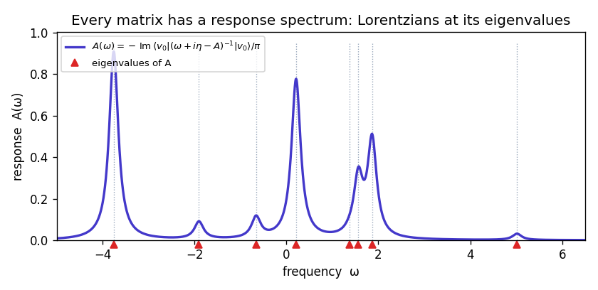
Evaluate the resolvent a hair above the real axis, at $z=\omega +i\eta$. Each pole softens, because $\mathrm{Im}\frac{1}{x+i\eta }=\frac{-\eta }{x^2+{\eta }^2}$ — a Lorentzian. The imaginary part of the resolvent is therefore a sum of Lorentzians, the spectral function:

The figure is this, computed on a random $8\times 8$ symmetric matrix (the same one from the continued-fraction page): a peak parked on every eigenvalue, with no physics anywhere in sight.

What a single peak tells you

Fit one Lorentzian to one peak and you read off three numbers, each a piece of physics. The center is the eigenvalue ${\lambda }_k$ — the resonant frequency, or in a quantum system the excitation energy. The area is the overlap weight $w_k$ — how brightly the probe couples to that mode, an oscillator strength. The width is the broadening $\eta$ — artificial for a discrete matrix, but in a system with damping it is the mode's inverse lifetime $\Gamma =1/\tau$. Fitting the isolated top peak above recovered all three: center $5.015$ (eigenvalue $5.017$), width $0.148$ ($\eta =0.12$), area $0.014$ (weight $0.011$).

Why every matrix has one

The Lorentzian shape is universal because it is nothing but the shape of a single pole $1/(\omega -\lambda +i\eta )$. Any matrix has eigenvalues, so any matrix has a resolvent with poles, so any matrix has a response spectrum — a graph Laplacian, a Markov generator, a random matrix, not just a Hamiltonian. That is the slightly strange part: the resonances are there whether or not the matrix means anything. When $A$ is a physical operator, those resonances become real spectral lines, and the three numbers above become real spectroscopy.

The full resolvent matrix

Everything above rode on a single number, $⟨v_0|(z1-A{)}^{-1}|v_0⟩$. But the resolvent is a whole matrix — that number is just one of its entries, the one you see from direction $v_0$. Sandwich it between two basis vectors instead and you get every element, exactly the way an operator is given a matrix in quantum mechanics:

Each entry carries different physics. The diagonal $R_{ii}$ is the local density of states — the spectrum seen from site $i$, the $⟨v_0|R|v_0⟩$ we used all along with $v_0$ a single site. The off-diagonal $R_{ij}$ is a propagator — the amplitude to travel from site $j$ to site $i$ at energy $z$ — and it decays with distance. The trace ${\sum }_i{R}_{ii}$ gathers every diagonal into the total density of states. Here is the whole matrix for a tight-binding chain, with the diagonal and the decaying first row read off:

# tight-binding chain, 6 sites; probe energy z = 3 (outside the band)
R = inv(z*I - A)             # the resolvent — a full 6x6 matrix, R_ij = <i|(zI-A)^-1|j>
[[ 0.382 -0.146  0.056 -0.021  0.008 -0.003]
 [-0.146  0.438 -0.167  0.064 -0.024  0.008]
 [ 0.056 -0.167  0.446 -0.170  0.064 -0.021]
 [-0.021  0.064 -0.170  0.446 -0.167  0.056]
 [ 0.008 -0.024  0.064 -0.167  0.438 -0.146]
 [-0.003  0.008 -0.021  0.056 -0.146  0.382]]

diag R_ii      = [0.382 0.438 0.446 0.446 0.438 0.382]   # local density of states
|R_0j|, j=0..5 = [0.382 0.146 0.056 0.021 0.008 0.003]   # propagator: decays with distance

The reason this object is hard to find under "resolvent" is that physics files it under a different name: it is the Green's function $G(z)=(z1-H{)}^{-1}$, and the $R_{ij}$ are its matrix elements, the propagators. Economou's Green's Functions in Quantum Physics is the standard reference; Haydock's recursion method is exactly the Lanczos continued fraction from this site applied to the local (diagonal) Green's function. The continuous cousin — a kernel $G(x,x^{\prime })$ instead of a matrix $G_{ij}$ — is the same object and lives on the Green's functions page.

The whole thing in code

The spectral function is a one-liner two ways: as an explicit sum of Lorentzians over the eigenpairs, or straight from the resolvent without ever diagonalizing. They agree to machine precision, and the spectral function integrates to one (a sum rule — all the weight has to live somewhere).

import numpy as np
# A: any symmetric matrix.  v0: a probe vector (unit norm).  eta: broadening.

lam, psi = np.linalg.eigh(A)
w = (v0 @ psi)**2                      # overlap weights: how much v0 "sees" each mode

def spectral(omega, eta):              # a sum of Lorentzians at the eigenvalues
    return np.sum(w * (eta/np.pi) / ((omega - lam)**2 + eta**2))

def spectral_from_resolvent(omega, eta):   # identical, straight from (z-A)^-1
    n = len(v0)
    G = v0 @ np.linalg.solve((omega + 1j*eta)*np.eye(n) - A, v0)
    return -G.imag / np.pi
# the two agree to machine precision; integral over omega is 1 (a sum rule).

Where it shows up

This is the hub the rest of the site's spectral machinery hangs from. Casida's equation computes the peak positions directly as eigenvalues; Liouville-Lanczos sweeps $\omega$ to draw the continuous $A(\omega )$ instead; the kernel polynomial method reconstructs the same curve from Chebyshev moments; and the Lanczos continued fraction is how you evaluate $A(\omega )$ for an operator far too large to diagonalize. Peak position is an energy, area is an intensity, width is a lifetime — the entire anatomy of an absorption spectrum, falling out of $1/(z-A)$.