The Hard-Sphere Fluid

Take everything away. No charges, no dipoles, no dispersion attraction, no springs — just impenetrable billiard balls of diameter $\sigma$ in a box. The potential is zero unless two spheres overlap, in which case it is infinite. There is no energy scale left, which means temperature can do nothing: every allowed configuration has exactly the same energy, and the Boltzmann factor is either 1 or 0. Whatever this system does, it does with entropy alone — and what it does is astonishing. It has a liquid-like fluid, a first-order phase transition, and a crystal, all from counting configurations.

That is why hard spheres are the hydrogen atom of liquids. Metropolis, Rosenbluth, Rosenbluth, Teller and Teller invented Markov chain Monte Carlo in 1953 on hard disks — this system, one dimension down — and the 1957 hard-sphere simulations of Alder and Wainwright and of Wood and Jacobson produced the first purely entropic freezing transition, a result so counterintuitive that a straw poll at a 1957 conference split roughly half against its existence. The coexistence densities settled at packing fractions ${\eta }_f\approx 0.494$ (fluid) and ${\eta }_m\approx 0.545$ (FCC crystal) by the thermodynamic-integration work of Hoover and Ree (1968).

The simulation: accept anything that fits

Metropolis Monte Carlo collapses to its minimal form here. Propose a small random displacement of one sphere; if it overlaps nothing, accept; if it overlaps anything, put it back. The Boltzmann factor $e^{-\beta \Delta U}$ is 1 or 0 — there is no energy to compute, ever:

@njit(cache=True)
def mc_sweeps(pos, L, nsweeps, dmax, seed):
    """Metropolis NVT for hard spheres (sigma = 1). Returns acceptance rate."""
    np.random.seed(seed)
    N = pos.shape[0]
    acc = 0
    for sweep in range(nsweeps):
        for _ in range(N):
            i = np.random.randint(N)
            trial = pos[i] + dmax * (np.random.random(3) - 0.5)
            trial -= L * np.floor(trial / L)          # periodic wrap
            ok = True
            for j in range(N):
                if j == i:
                    continue
                d = trial - pos[j]
                d -= L * np.round(d / L)              # minimum image
                if d[0]*d[0] + d[1]*d[1] + d[2]*d[2] < 1.0:
                    ok = False                        # overlap: reject
                    break
            if ok:
                pos[i] = trial                        # no overlap: accept
                acc += 1
    return acc / (nsweeps * N)

Everything below runs $N=500$ spheres started on an FCC lattice, equilibrated for 2,000 sweeps and measured over 12,000, at packing fractions from $\eta =0.05$ to 0.47 — just short of freezing.

Two pressures, no forces

A hard-sphere pressure cannot come from summing forces — the force is a delta function at contact. The equation of state has to be measured structurally, and the cross-check is that two completely different routes agree:

Route 1 — the contact value. The virial theorem for hard spheres collapses to an exact statement about the pair correlation function at contact:

Histogram $g(r)$ (the subject of its own page), extrapolate to $r=\sigma$ from above, and the pressure falls out of pure structure.

Route 2 — virtual compression. Shrink the box (and every coordinate) by a factor $s$ just below 1 and ask: would any pair now overlap? The acceptance probability of this virtual volume move gives the excess pressure directly, $\beta p_{ex}=-\ln ⟨P_{acc}⟩/\Delta V$ (Eppenga & Frenkel's trick). No force, no contact extrapolation — just the question "does it still fit?"

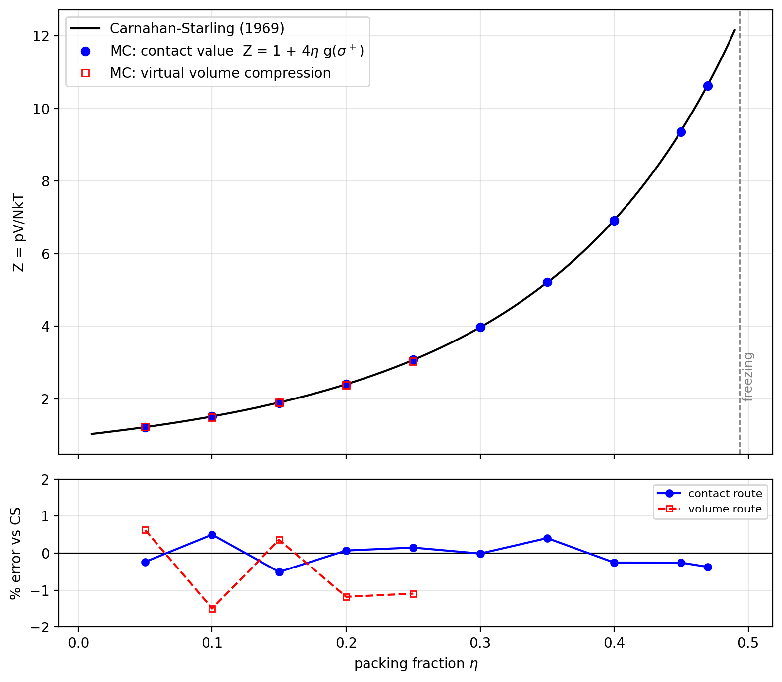
Both routes, against the Carnahan-Starling equation of state (1969) — the famous closed form built by noticing the virial coefficients are nearly integers and resumming the guessed pattern:

eta=0.05  Z_contact=1.2246 (-0.23%)  Z_vol=1.2351 (+0.62%)  CS=1.2274  p_ins=6.436e-01  mu_ex=0.441 (CS 0.441)
eta=0.10  Z_contact=1.5289 (+0.50%)  Z_vol=1.4985 (-1.49%)  CS=1.5213  p_ins=3.760e-01  mu_ex=0.978 (CS 0.978)
eta=0.15  Z_contact=1.8941 (-0.51%)  Z_vol=1.9105 (+0.36%)  CS=1.9037  p_ins=1.934e-01  mu_ex=1.643 (CS 1.641)
eta=0.20  Z_contact=2.4080 (+0.07%)  Z_vol=2.3779 (-1.18%)  CS=2.4062  p_ins=8.388e-02  mu_ex=2.478 (CS 2.469)
eta=0.25  Z_contact=3.0787 (+0.15%)  Z_vol=3.0405 (-1.09%)  CS=3.0741  p_ins=2.946e-02  mu_ex=3.525 (CS 3.519)
eta=0.30  Z_contact=3.9733 (-0.01%)  Z_vol=4.1067 (+3.35%)  CS=3.9738  p_ins=7.482e-03  mu_ex=4.895 (CS 4.872)
eta=0.35  Z_contact=5.2269 (+0.41%)  Z_vol=5.1500 (-1.07%)  CS=5.2057  p_ins=1.261e-03  mu_ex=6.676 (CS 6.650)
eta=0.40  Z_contact=6.9084 (-0.25%)  Z_vol=dead (P_acc -> 0)  CS=6.9259  p_ins=1.075e-04  mu_ex=9.138 (CS 9.037)
eta=0.45  Z_contact=9.3608 (-0.25%)  Z_vol=dead (P_acc -> 0)  CS=9.3847  p_ins=5.000e-06  mu_ex=12.206 (CS 12.327)
eta=0.47  Z_contact=10.6208 (-0.37%)  Z_vol=dead (P_acc -> 0)  CS=10.6603  p_ins=4.167e-07  mu_ex=14.691 (CS 13.994)

Read the two routes separately. The contact route tracks Carnahan-Starling within half a percent all the way to freezing. The volume route agrees with it at low and moderate density — genuinely independent confirmation — and then dies above $\eta \approx 0.35$: a global compression of a dense configuration is rejected essentially every time, the acceptance probability underflows, and the estimator returns nothing rather than something wrong. That is the same exponential death the Widom method suffers below, and it is the recurring failure mode of every "count rare successes" estimator in this subject. Note also what $Z$ does not depend on: temperature. For hard spheres $Z(\eta )$ is the entire thermodynamics — $pV/N{k}_{B}T$ is a function of density alone, because there is no energy scale to compare $k_{B}T$ against.

Widom insertion: the chemical potential from ghosts

Widom (1963) noticed that the excess chemical potential — the free-energy cost of adding one more particle — is an average you can measure without ever actually adding it: $\beta {\mu }_{ex}=-\ln ⟨e^{-\beta \Delta U}⟩$, where $\Delta U$ is the energy a randomly placed ghost particle would feel. For hard spheres the exponential is again 1 or 0, so the whole method reduces to: throw darts, count the fraction that land in a sphere-sized hole.

@njit(cache=True)
def widom_insertions(pos, L, ntrials, seed):
    """Fraction of random ghost insertions that create no overlap."""
    np.random.seed(seed)
    hits = 0
    for _ in range(ntrials):
        t = np.random.random(3) * L                  # a ghost sphere, anywhere
        ok = True
        for j in range(pos.shape[0]):
            d = t - pos[j]
            d -= L * np.round(d / L)
            if d[0]*d[0] + d[1]*d[1] + d[2]*d[2] < 1.0:
                ok = False
                break
        if ok:
            hits += 1
    return hits / ntrials                            # <e^(-beta dU)> = P(no overlap)

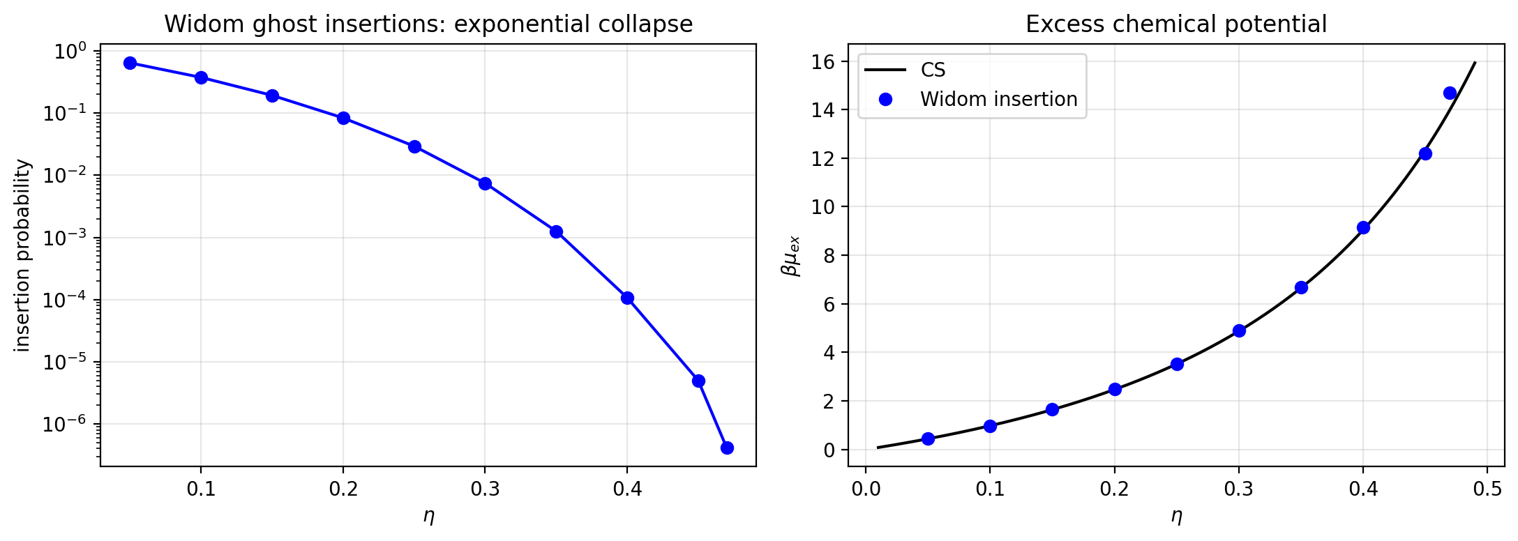
The right panel is the success: $\beta {\mu }_{ex}$ tracks the Carnahan-Starling prediction across the whole fluid. The left panel is the built-in failure mode, and it is worth staring at: the insertion probability falls roughly exponentially with density, into the 10^-5 range by $\eta =0.47$. Every decade costs ten times the statistics. Push much past freezing and no laptop lifetime of darts will find a hole — which is precisely why staged-insertion and thermodynamic-integration methods exist. A method whose error bars tell you when it stops working is a good method.

Reproduce it

scripts/gen_hard_spheres.py regenerates every number and figure on this page and the radial distribution function page in one run (numba does the heavy lifting). The natural next steps in the stat-mech plan: event-driven hard-sphere molecular dynamics — no timestep, jump collision to collision — and jamming, where packings this page politely stops short of get compressed until they lock. Related pages already live: Lennard-Jones MD, Wang-Landau, critical exponents from finite-size scaling.