The Radial Distribution Function

Stand on any particle in a fluid and count neighbors in a thin shell at distance $r$. Divide by the count an ideal gas at the same density would give you. That ratio is the radial distribution function $g(r)$ — the conditional probability of finding a particle at $r$ given one at the origin, relative to pure chance. It is the single most information-dense curve in liquid-state physics: scattering experiments measure it, integral-equation theories predict it, and — for hard spheres — the entire equation of state hides inside one of its values.

Histogramming it without fooling yourself

The measurement is a pair-distance histogram; all the physics care goes into the normalization, which is where first implementations reliably go wrong. Work it from the smallest case up. One tagged particle, ideal gas: the expected count in a shell is density times shell volume, $\rho \cdot 4\pi r^{2}dr$. Now count over all $N(N-1)/2$ distinct pairs instead of around one tagged particle: that is $N/2$ tagged-particle experiments at once, so the ideal count becomes $(N/2)\rho 4\pi r^{2}dr$. Divide the measured histogram by that, and the two classic bugs — a factor of 2 from pair counting, and using $r$ at the bin edge instead of the bin center — are both dodged:

@njit(cache=True)
def gr_histogram(pos, L, bins, rmax):
    """Accumulate pair-distance histogram (all pairs, counted once)."""
    N = pos.shape[0]
    hist = np.zeros(bins)
    dr = rmax / bins
    for i in range(N - 1):
        for j in range(i + 1, N):
            d = pos[i] - pos[j]
            d -= L * np.round(d / L)          # minimum image
            r = np.sqrt(d[0]*d[0] + d[1]*d[1] + d[2]*d[2])
            if r < rmax:
                hist[int(r / dr)] += 1.0
    return hist

# normalization: divide by the pair count an IDEAL GAS would put in each shell
r_mid = (np.arange(bins) + 0.5) * dr
shell = 4 * np.pi * r_mid**2 * dr             # shell volume
g = (hist / nsamp) / (0.5 * N * rho * shell)  # N/2 ordered pairs x rho x shell

Sanity anchors before trusting any curve: $g(r)=0$ inside the core (hard spheres cannot interpenetrate), $g(r)\to 1$ at large $r$ (far away, the fluid forgets you exist — no normalization fudging allowed), and for an ideal gas the whole curve is 1 everywhere.

Against an analytic answer: Percus-Yevick

Hard spheres are one of the very few systems where an integral-equation theory can be solved in closed form. The Percus-Yevick closure of the Ornstein-Zernike equation was cracked independently by Wertheim and by Thiele in 1963: the direct correlation function $c(r)$ is a cubic polynomial inside the core and zero outside. 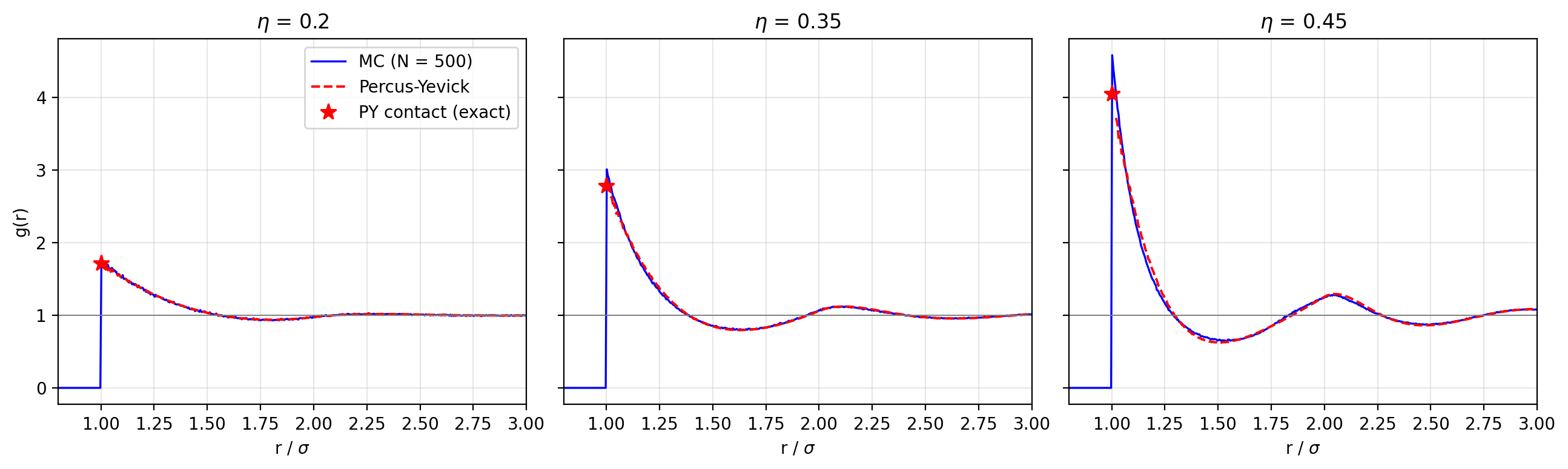Fourier transform, apply OZ, transform back, and the theoretical $g(r)$ emerges — no simulation, just 1960s algebra. Overlaid on the Monte Carlo histograms from the hard-sphere fluid page at three densities:

PY inversion check at eta=0.35: extrapolated g(sigma+) = 2.7288 vs analytic 2.7811 (-1.88%)

LJ g(r) first peak: 3.006 at r = 1.083

At $\eta =0.20$ theory and simulation are indistinguishable. By $\eta =0.45$ the PY curve visibly underestimates the contact peak — a known, systematic shortcoming: PY's two thermodynamic routes (virial and compressibility) disagree with each other at high density, bracketing the truth, and the Carnahan-Starling equation of state is in essence their weighted average. Watching an approximate theory fail in a characterized, documented way is worth more than watching it succeed.

Pressure from structure alone

For hard spheres the virial theorem reduces to the contact-value theorem,

so extrapolating these histograms to $r\to {\sigma }^{+}$ (a quadratic fit over the first few bins) hands you the full equation of state — which is exactly how route 1 on the equation-of-state page reproduced Carnahan-Starling at the percent level. For this system, structure is thermodynamics: one curve, measured by counting neighbors, contains the pressure at every density.

What attraction adds: the Lennard-Jones contrast

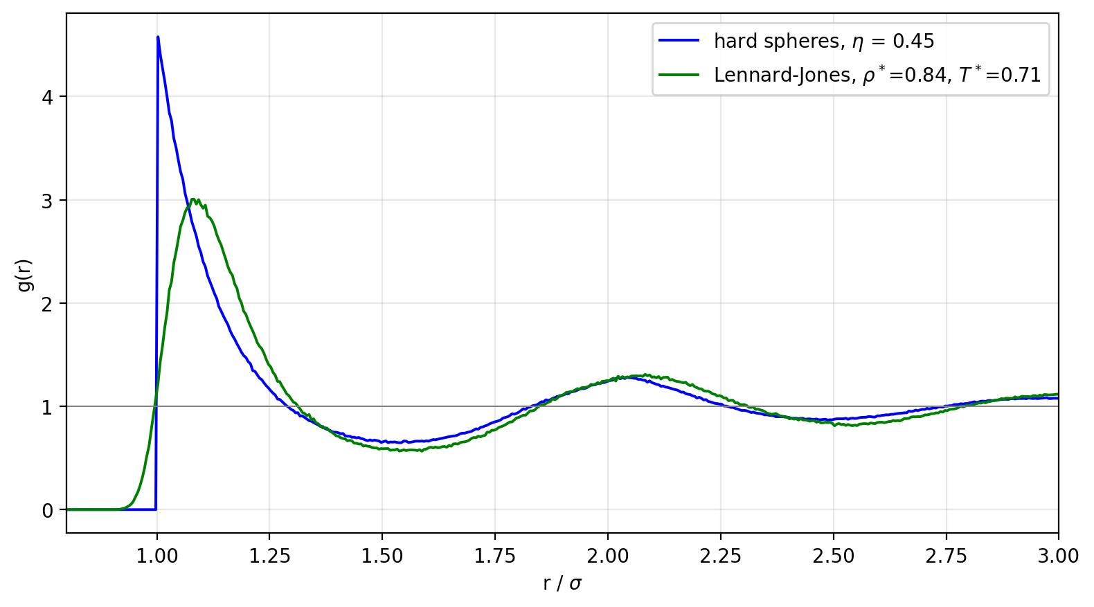
A dense Lennard-Jones liquid near its triple point against hard spheres at comparable packing: the oscillations — first shell, depletion ring, second shell — are nearly the same, because packing geometry, not attraction, dictates liquid structure. That observation is the seed of the van der Waals picture and of perturbation theories of liquids (Weeks-Chandler-Andersen): treat the liquid as hard spheres for structure, add attraction as a correction for energetics. The visible differences are the signatures of the well: the LJ first peak sits near the potential minimum rather than jammed against contact, and it is taller — particles are not merely allowed to touch, they are invited.

What experiments see

X-ray and neutron scattering measure the static structure factor $S(k)$, which is the Fourier transform of $g(r)-1$: the scattered intensity at wavevector $k$ interrogates density correlations at wavelength $2\pi /k$. Every measured $g(r)$ of a simple liquid — argon from neutrons, colloids from confocal microscopy — shows the shell structure above. In the measurement-to-model language used across this site: $S(k)$ is what the detector records, $g(r)$ is the model-side object, and the Fourier pair is the bridge.

Reproduce it

Every curve here comes from the same run as the equation-of-state page: scripts/gen_hard_spheres.py, including the PY inversion (validated against the exact PY contact value $g({\sigma }^{+})=(1+\eta /2)/(1-\eta {)}^2$ before being trusted with anything else — with one instructive wrinkle: evaluating the numerically inverted $g(r)$ at the contact discontinuity returns the jump's midpoint, because a truncated Fourier reconstruction of a step converges to the average of the two sides. The check therefore extrapolates from just outside, the same way the MC contact value is extracted, and lands within 2% of the closed form.