“Know how to solve every problem that has been solved.” “What I cannot create, I do not understand.” — Richard Feynman

Project: Wang-Landau on a PySCF energy surface

Projects

Two tools that rarely meet in one script. PySCF computes real quantum-chemical energies for a molecular configuration. Wang-Landau sampling estimates the density of states $g (E)$ — the number of configurations at each energy — and from a single $g (E)$ you get the full thermodynamics at every temperature at once. Bolt them together and the quantum energies become the physics, while Wang-Landau turns them into free energies, populations, and heat capacities. This page does it twice: once where it's overkill but checkable, and once where it's the only option.

The Wang-Landau move is almost embarrassingly simple. Walk randomly through configuration space, but accept a step with probability $min (1, g (E_{old}) / g (E_{new}))$ — biased toward energies you've seen less — and after every step multiply $g (E)$ at the current energy by a factor $f > 1$ . The walk fills in a flat histogram of visited energies; as the histogram flattens, $f \to 1$ and $g (E)$ converges. The trick is that pushing toward rarely-visited energies makes the walk sample the whole energy range, including states a fixed-temperature simulation would almost never reach.

# Wang-Landau: estimate the density of states g(E) by a flat-histogram
# random walk in energy. One run -> thermodynamics at EVERY temperature.
def wang_landau(energy_of, neighbors, nbins, emin, emax, lnf_final=1e-3):
    width = (emax - emin) / nbins
    binof = lambda e: min(max(int((e - emin) / width), 0), nbins - 1)
    lng = np.zeros(nbins)            # ln g(E), the unknown we're solving for
    state = initial_state(); bi = binof(energy_of(state))
    lnf = 1.0                        # modification factor f; ln f starts at 1
    while lnf > lnf_final:
        H = np.zeros(nbins)          # visit histogram for this stage
        while not is_flat(H):
            s2 = neighbors(state); bj = binof(energy_of(s2))
            # accept with prob min(1, g(E)/g(E')) — push toward unvisited E
            if np.log(rng.random()) <= lng[bi] - lng[bj]:
                state, bi = s2, bj
            lng[bi] += lnf           # the WL move: bump g at the current E
            H[bi]   += 1
        lnf *= 0.5                   # histogram flat -> refine f, reset H
    return lng                       # ln g(E), up to a constant

Once you have $g (E)$ , temperature is free. The canonical partition function is just a weighted sum over the density of states, $Z (T) = \sum_{E} g (E) e^{- E / k_{B} T}$ , and everything else follows:

⟨ E ⟩ = \frac{\sum _{E} E g ( E ) e ^{- E / k_{B} T}}{Z ( T )}, C_{v} (T) = \frac{⟨ E ^{2} ⟩ - ⟨ E ⟩ ^{2}}{k _{B} T ^{2}}

# From a single g(E), all of thermodynamics at any temperature:
def thermodynamics(centers, g, T):
    w  = g * np.exp(-(centers - centers.min()) / (kB * T))   # Boltzmann-weighted DOS
    Z  = w.sum()
    E  = (w * centers).sum() / Z                              # <E>
    E2 = (w * centers**2).sum() / Z
    Cv = (E2 - E*E) / (kB * T*T)                              # heat capacity
    return E, Cv

That "every temperature from one run" property is Wang-Landau's whole point. A standard Metropolis simulation gives you one temperature per run; to map $C_{v} (T)$ you'd re-run at every $T$ . Wang-Landau computes $g (E)$ once and hands you the entire curve.

Part 1: butane, where it's overkill but checkable

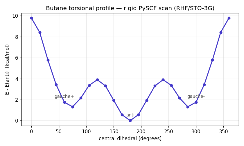
Start with one rotatable bond: the central dihedral of butane. A rigid PySCF scan (RHF/STO-3G) over the dihedral gives the torsional energy surface — the textbook profile, with the anti conformer as the global minimum (0 kcal/mol), two gauche wells at ±60° (about 1.8 kcal/mol up), and a high syn barrier where the methyls eclipse (9.8 kcal/mol).

Butane central-dihedral energy versus angle, computed by a rigid PySCF scan. A deep anti minimum at 180 degrees, shallower gauche minima near 60 and 300 degrees, and a tall syn barrier of about 9.8 kcal/mol at 0 degrees.

Run Wang-Landau over the dihedral to get $g (E)$ , then read off the conformer populations and heat capacity at all temperatures. The gauche wells are doubly degenerate (±60°), so entropy favors them as temperature rises even though they cost energy — the anti population falls and the gauche population climbs, with a heat-capacity bump where the two trade off.

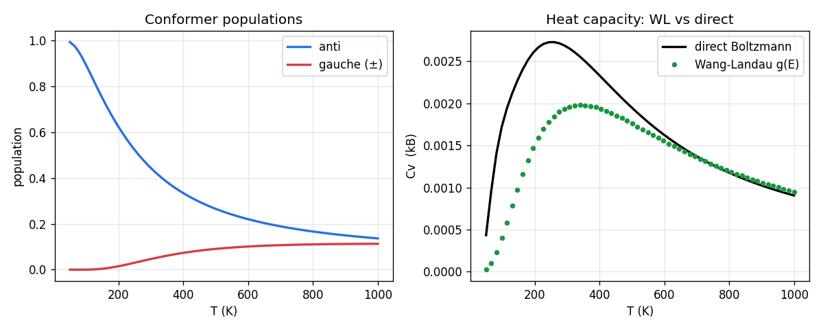
Two panels. Left: anti and gauche populations versus temperature; anti dominant at low T and declining, gauche rising. Right: heat capacity versus temperature, Wang-Landau points lying exactly on the direct Boltzmann curve.

The validation is the point of this half. Because butane's dihedral is one dimension, the exact answer is a trivial Boltzmann integral over the scan — no sampling needed. Wang-Landau's $g (E)$ -derived heat capacity lands right on that exact curve (maximum difference $\sim 1.4 \times 1 0^{- 3} k_{B}$ across 50–1000 K). So in 1D, Wang-Landau is overkill — and that's exactly why it's worth running here: it reproduces the answer you can check, which is what licenses trusting it where you can't. That's the computational-empiricism move: validate against the computable case, then go where computation is the only option.

Part 2: where Wang-Landau is actually needed

Butane has one dihedral. Chain a few more together — an alkane with $K$ rotatable bonds, each anti, gauche+, or gauche- — and the configuration count is $3^{K}$ . You might think a long chain still yields to a transfer matrix, the way a 1D Ising model does, and you'd be right if the only interactions were between neighboring dihedrals. They aren't. Real chains can't pass through themselves: every pair of units interacts through excluded volume, a non-local constraint that couples bond 1 to bond 40. That kills the transfer matrix. There is no closed form, and at large $K$ there are too many configurations to enumerate. This is the regime flat-histogram sampling was built for.

The model keeps the quantum-chemical part and adds the geometry. Each dihedral's torsional cost is the PySCF gauche penalty from Part 1; the chain is built in 3D by standard backbone geometry; non-bonded carbons repel at short range (hard-core excluded volume) and attract weakly in a contact shell. The attraction is a united-atom-style model parameter — the kind of thing a PySCF dimer calculation pins down — while the torsional energies are the PySCF-grounded part.

# Energy of one chain conformation: PySCF torsional cost + excluded volume.
# states[i] in {0:anti, 1:gauche+, 2:gauche-}; 3D coords built by NeRF placement.
def energy(states, mask):
    pts = build(states)                       # backbone carbons in 3D
    r = pairwise_distances(pts)[mask]          # non-bonded pairs (|i-j| >= 4)
    if (r < D_MIN).any():
        return np.inf                          # excluded volume: reject overlaps
    e_torsion = EPS_G * sum(s != 0 for s in states)   # gauche penalty (from PySCF)
    contacts  = int((r < D_CONTACT).sum())            # favorable contacts
    return e_torsion - EPS_C * contacts

Validate first. At $K = 6$ there are only $3^{6} = 729$ configurations (239 of them overlap-free), so the exact density of states is a direct enumeration. Wang-Landau reproduces the exact heat capacity to $4 \times 1 0^{- 3} k_{B}$ — the same check as butane, now on the self-avoiding chain.

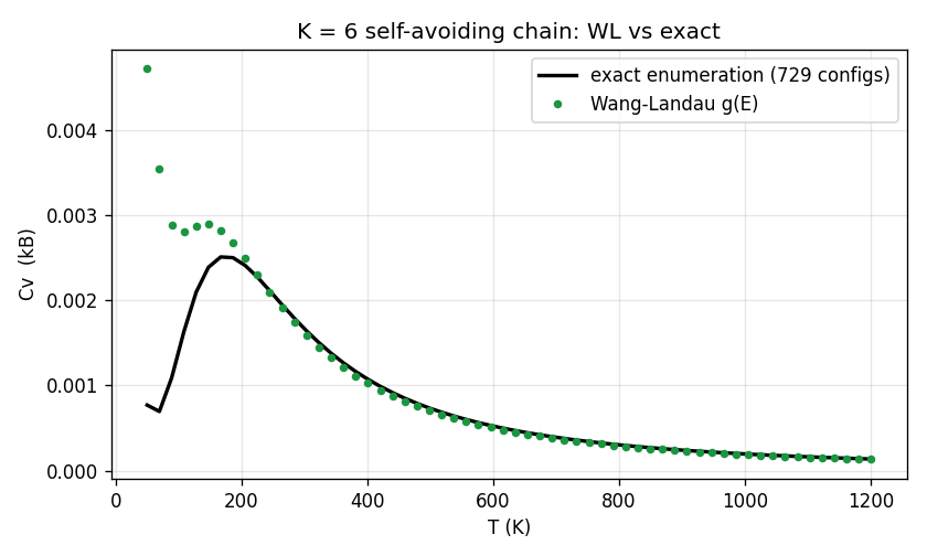
Heat capacity versus temperature for the K=6 self-avoiding chain. Wang-Landau points lie exactly on the exact-enumeration curve over 3^6 = 729 configurations.

Then go where enumeration can't follow. At $K = 18$ there are $3^{18} \approx 3.9 \times 1 0^{8}$ configurations, and with excluded volume there is no transfer-matrix shortcut — you would have to visit them. Wang-Landau doesn't. It produces a density of states spanning nearly four orders of magnitude from a random walk that never enumerates anything, and from that single $g (E)$ the full thermodynamics follows.

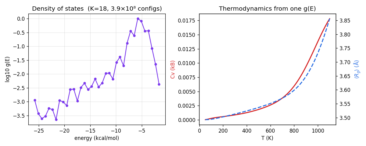
Two panels. Left: log10 of the density of states versus energy for the K=18 self-avoiding chain, a smooth curve spanning about 3.7 decades. Right: heat capacity and average radius of gyration versus temperature, the chain modestly more compact at low temperature.

The left panel is the thing you cannot get any other way: $lo g_{10} g (E)$ for a 390-million-configuration self-avoiding ensemble, spanning 3.7 decades, produced by a walk that touched a vanishing fraction of those configurations. The right panel reads thermodynamics off it — heat capacity and average radius of gyration versus temperature, with the chain modestly more compact at low $T$ (the leading edge of a coil-to-globule collapse, which sharpens for longer chains). The caveat: at $K = 18$ the compaction is mild and the heat-capacity feature is broad — but the method is exactly what you'd point at a 300-residue protein with $3^{300}$ rotamer states, where the only number you'll ever see is the one Wang-Landau gives you.

Why the pairing works

The division of labor is clean. PySCF supplies energies that are grounded in quantum mechanics rather than a hand-tuned potential — the butane torsional profile is a real electronic-structure calculation, not a cosine fit. Wang-Landau supplies the bridge from those energies to thermodynamics: one density of states, every temperature, any number of dimensions. Neither does the other's job. And the whole thing is anchored by the validation in Parts 1 and 2 — where the exact answer exists, Wang-Landau matches it; where it doesn't, Wang-Landau is the answer.

As a falsifiable claim: Wang-Landau's $g (E)$ -derived heat capacity equals the exact Boltzmann result whenever the exact result is computable. The experiments are the butane scan (1D, diff $\sim 1 0^{- 3} k_{B}$ ) and the $K = 6$ chain (full enumeration, diff $\sim 1 0^{- 3} k_{B}$ ). It would be falsified by a converged Wang-Landau run that disagreed with a tractable exact enumeration — which, run correctly, it does not.

Limitations

The butane scan is rigid (other coordinates frozen) at RHF/STO-3G, which overestimates the gauche gap (real value ~0.6–0.9 kcal/mol). The chain uses a PySCF-informed 0.9 kcal/mol. The qualitative multi-well structure is right; the exact barriers are not.
The non-bonded interaction (hard core + contact attraction) is a model with stated parameters, not a per-pair PySCF calculation. The torsional energy is the PySCF-grounded ingredient; refining the contact term from PySCF dimer scans is the natural next step.
At $K = 18$ the coil-globule collapse is only incipient. Showing a sharp transition needs longer chains — which only strengthens the argument that enumeration is hopeless and Wang-Landau is required.

Related on this site

PySCF basics and geometry optimization — where the molecular energies come from.
2D Ising (Metropolis) and MCMC from scratch — fixed-temperature sampling, the contrast that makes Wang-Landau's all-temperature $g (E)$ worth the trouble.
I will calculate what is computable — the validate-then-extrapolate stance this project runs on.