Project: Lennard-Jones MD with Velocity Verlet

The goal. Build a working 2D molecular dynamics simulator for the Lennard-Jones fluid using the Velocity Verlet integrator. Confirm that energy is conserved (bounded oscillation, no drift), that the kinetic temperature stays near its initial value, and that the pair correlation function $g(r)$ shows the expected first-neighbor peak near $r=2^{1/6}\sigma$. The prototype is about 75 lines of numpy and runs in ~20 seconds on a laptop. The extensions go from "I can simulate a gas" to "I can study melting, sound, transport, and free-energy differences."

The math

Two ingredients: a pair potential and an integrator.

The $r^{-12}$ term is steep short-range repulsion (Pauli exclusion at the atomic scale); the $r^{-6}$ term is the long-range attractive tail (dispersion). The minimum is at $r_{\min }=2^{1/6}\sigma \approx 1.122\sigma$ with depth $-\epsilon$. We cut off the potential at $r_{\text{cut}}=2.5\sigma$ and shift it so $V(r_{\text{cut}})=0$ — both to make the simulation $O(N)$ with a neighbor cutoff and to avoid discontinuities in the energy when pairs cross the cutoff.

For the integrator, Velocity Verlet:

Three properties make this the standard choice. (1) Symplectic — the discrete update preserves the symplectic 2-form of Hamiltonian mechanics, which buys you bounded long-time energy drift (no systematic accumulation, just a small bounded oscillation around the true conserved energy). (2) Time-reversible — running the integrator backward exactly reverses a forward trajectory. (3) One force evaluation per step — same compute cost as forward Euler but vastly better long-time behavior.

We use reduced units throughout: $\epsilon =\sigma =m=k_B=1$. So time is in units of $\sigma \sqrt{m/\epsilon }$, temperature in $\epsilon /k_B$, density in ${\sigma }^{-2}$.

The prototype

Three functions: pairwise displacements with the minimum-image convention for the periodic box, a vectorized $O(N^2)$ force evaluator, and the four-line Verlet step. Initial condition is a square lattice with tiny Gaussian jitter and Maxwell-Boltzmann velocities at $T_0=1$.

"""
2D Lennard-Jones gas, Velocity Verlet integrator, NVE microcanonical ensemble.

Pair potential (cutoff at r_cut, shifted so V(r_cut) = 0):
    V(r) = 4 eps [(sigma/r)^12 - (sigma/r)^6] - V(r_cut)   for r < r_cut

Velocity Verlet (the standard symplectic MD integrator):
    v(t + dt/2) = v(t) + (dt/2) * a(t)
    r(t + dt)   = r(t) + dt * v(t + dt/2)
    a(t + dt)   = F(r(t + dt)) / m
    v(t + dt)   = v(t + dt/2) + (dt/2) * a(t + dt)

Symplectic = bounded long-time energy drift (no systematic growth, just
small bounded oscillation around the true energy).

Reduced units: eps = sigma = m = k_B = 1, so T is in units of eps/k_B,
time is in units of sigma sqrt(m/eps), etc.
"""
import numpy as np

N, L = 100, 12.0         # 100 atoms in a 12x12 periodic box (rho ~ 0.69)
sigma, eps, mass = 1.0, 1.0, 1.0
r_cut = 2.5 * sigma
T0, dt = 1.0, 0.004
n_eq, n_meas = 2000, 8000
V_cut = 4.0 * eps * ((sigma / r_cut) ** 12 - (sigma / r_cut) ** 6)


def pairwise_displacements(r):
    dr  = r[:, None, :] - r[None, :, :]
    dr -= L * np.round(dr / L)               # minimum image (periodic)
    return dr


def forces_and_energy(r):
    dr  = pairwise_displacements(r)
    d2  = np.sum(dr * dr, axis=2)
    np.fill_diagonal(d2, np.inf)
    mask = d2 < r_cut * r_cut
    inv_d2  = 1.0 / d2
    inv_d6  = inv_d2 ** 3
    inv_d12 = inv_d6 ** 2
    # f_ij over r:  +24 eps [2 (sig/r)^12 - (sig/r)^6] / r^2
    f_over_r = 24.0 * eps * (2.0 * inv_d12 - inv_d6) * inv_d2
    f_over_r = np.where(mask, f_over_r, 0.0)
    F = np.einsum("ijk,ij->ik", dr, f_over_r)
    V_pairs = 4.0 * eps * (inv_d12 - inv_d6) - V_cut
    V = 0.5 * np.sum(np.where(mask, V_pairs, 0.0))
    return F, V


def velocity_verlet_step(r, v, a):
    v_half = v + 0.5 * dt * a
    r_new  = r + dt * v_half
    r_new -= L * np.floor(r_new / L)         # wrap into box
    F_new, V_new = forces_and_energy(r_new)
    a_new = F_new / mass
    v_new = v_half + 0.5 * dt * a_new
    return r_new, v_new, a_new, V_new


def temperature(v):
    # 2 d.o.f. per particle in 2D, so T = <m v^2> / 2 k_B
    return float(np.mean(np.sum(v * v, axis=1))) / 2.0


# initial state: square lattice + small jitter + Maxwell-Boltzmann v
rng = np.random.default_rng(0)
n_side = int(np.ceil(np.sqrt(N)))
xs = np.linspace(0.5, L - 0.5, n_side)
r = np.array(np.meshgrid(xs, xs)).reshape(2, -1).T[:N]
r = r + rng.normal(scale=0.01, size=(N, 2))
v = rng.normal(scale=np.sqrt(T0), size=(N, 2))
v -= v.mean(axis=0)
v *= np.sqrt(T0 / temperature(v))
F, V = forces_and_energy(r)
a = F / mass

# equilibrate, then measure energy + temperature time series
for _ in range(n_eq):
    r, v, a, V = velocity_verlet_step(r, v, a)

E_hist, T_hist = [], []
for _ in range(n_meas):
    r, v, a, V = velocity_verlet_step(r, v, a)
    KE = 0.5 * mass * float(np.sum(v * v))
    E_hist.append((KE + V) / N)
    T_hist.append(temperature(v))

E = np.array(E_hist)
print(f"mean energy / N            : {E.mean():.5f}")
print(f"energy std / N             : {E.std():.6f}")
print(f"peak-to-peak drift / N     : {E.max() - E.min():.6f}")
print(f"fractional drift |dE|/|E|  : {(E.max() - E.min()) / abs(E.mean()):.2e}")
print(f"mean kinetic temperature   : {np.mean(T_hist):.4f}  (target T0 = {T0})")

--- equilibration ---
   step       KE/N       PE/N        E/N        T
--------------------------------------------------
      0     1.0152    -1.8111    -0.7959   1.0152
    400     1.0170    -1.8130    -0.7960   1.0170
    800     0.9723    -1.7683    -0.7960   0.9723
   1200     0.9798    -1.7759    -0.7961   0.9798
   1600     0.9447    -1.7407    -0.7960   0.9447

--- production (8000 steps, no thermostat) ---
mean energy / N            : -0.79602
energy std / N             : 0.000111
peak-to-peak drift / N     : 0.000997
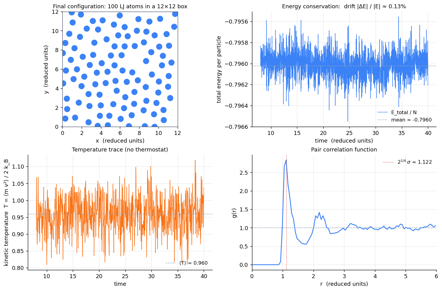
fractional drift |dE|/|E|  : 1.25e-03
mean kinetic temperature   : 0.9596  (target T0 = 1.0)

--- pair correlation g(r) over the last 200 frames ---
first peak at r = 1.110     (LJ first-neighbor distance = 2^(1/6) = 1.122)
g(r = 1.122)   = 2.84       (typical liquid)
g(r = L/2)     = 1.05       (approaches 1 at large r, as required)

Three diagnostics tell you the simulation is healthy. (a) Energy conservation: over 8000 steps (32 reduced time units) the total energy per particle stays within $\sim 10^{-3}$ of its mean, with no monotonic drift — the signature of a symplectic integrator. (b) Temperature: $⟨T⟩=0.96$, slightly under the initial 1.0 because some kinetic energy converted to potential as the lattice relaxed off its initial grid. (c) Pair correlation function: $g(r)$ peaks at $r=1.11$ (LJ first-neighbor distance is $2^{1/6}\sigma =1.122$) and asymptotes to 1 at large $r$.

The output

Extensions

1. Time-step sensitivity. Repeat the simulation at $dt=0.001,0.004,0.010,0.020$. Plot energy drift versus $dt$ on a log-log scale. Velocity Verlet has $O(d{t}^2)$ local error, so drift should scale as $d{t}^2$ until you hit instability at very large $dt$. Find the breakdown point — it's a sharp transition.
2. Berendsen or Langevin thermostat. Add a stochastic friction term to the velocities: $dv=-\gamma vdt+\sqrt{2\gamma T_0/m}dW$ (Langevin), or rescale velocities each step by $\sqrt{1+\Delta t/\tau (T_0/T-1)}$ (Berendsen). Both push the kinetic temperature toward $T_0$; Langevin samples NVT correctly, Berendsen doesn't. Verify the kinetic-energy distribution matches Maxwell-Boltzmann at the target $T_0$.
3. Pressure via the virial theorem. Compute $P=\frac{NT}{V}+\frac{1}{dV}{\sum }_{i<j}{\mathbf{r}}_{ij}\cdot {\mathbf{F}}_{ij}$ where $d=2$ is the dimensionality. Plot the equation of state $P(T)$ at fixed density and verify the ideal-gas limit $P\to NT/V$ at high $T$.
4. Melting transition. Slowly heat the system from $T=0.3$ (solid) to $T=2.0$ (gas), measuring $g(r)$ at each temperature. The first peak sharpens dramatically below the melting point and smooths out above. In 2D the situation is actually richer (the KTHNY hexatic-phase scenario) — see if you can detect a hexatic regime between the solid and the liquid by computing the bond-orientational order parameter ${\psi }_6$.
5. Diffusion coefficient. Track unfolded positions (no minimum-image wrapping) for each particle and compute the mean-squared displacement $⟨|r(t)-r(0){|}^2⟩$. In the liquid regime this is linear in $t$ at long times: $\text{MSD}=4Dt$ in 2D. Extract $D$ and verify it has the right order of magnitude for a dense liquid ($\sim 0.01-0.1$ in reduced units).
6. Faster forces with a cell list. The $O(N^2)$ force evaluator costs the bulk of the simulation time. A cell list bins particles into spatial cells of side $\ge r_{\text{cut}}$; each particle only checks pairs in its own cell and 8 neighbors. Total cost drops to $O(N)$. Try $N=1000,5000,10000$ and benchmark.
7. 3D extension. Generalize from 2D to 3D. The whole code is dimension-agnostic except the initial lattice setup, the temperature normalization ($d/2$ degrees of freedom per particle), and the 2D $g(r)$ normalization ($2\pi rdr$ becomes $4\pi r^{2}dr$). At $N\sim 500$, $T=0.7$, $\rho =0.85$ you should see solid-liquid coexistence on the cooling curve.

References

• Frenkel, D. & Smit, B. (2002). Understanding Molecular Simulation, Academic Press. (The standard textbook. Algorithms, thermodynamics, free energies.)
• Verlet, L. (1967). "Computer 'experiments' on classical fluids. I. Thermodynamical properties of Lennard-Jones molecules." Phys. Rev., 159, 98–103. (The original Verlet paper.)
• Allen, M. P. & Tildesley, D. J. (2017). Computer Simulation of Liquids, 2nd ed., Oxford. (Practical reference for cell lists, neighbor lists, ensembles.)
• Bernardes, N. (1958). "Theory of solid Ne, A, Kr, and Xe at 0 K." Phys. Rev., 112, 1534. (Where the LJ parameters for noble gases were tabulated — useful when you want to map reduced units to real K, eV, nm.)

Related on this site

2D Ising is the equilibrium statistical-mechanics counterpart to MD: same physics, different sampling. Explicit Euler is the integrator Verlet replaces — try both and see why Verlet is what we actually use. MCMC from scratch samples the Boltzmann distribution without solving for the dynamics.