Project: GPU-Accelerated Ising Monte Carlo

The same Metropolis sweep on GPU and CPU — validated against Onsager, then timed. Stack: Python · PyTorch · Metal / MPS (CUDA-portable).

What this is

The 2D Ising model is the natural first GPU workload: the physics is exact (Onsager solved it in 1944), and the update is embarrassingly parallel. This project runs a batched checkerboard Metropolis Monte Carlo — many independent lattices, at many temperatures, all sweeping at once — on the GPU, then does the two things that make it worth showing: it reproduces Onsager, and it is measurably faster than a well-optimized CPU baseline. The code is device-agnostic; it runs on Apple's Metal backend here and on CUDA elsewhere by changing one string.

import torch

def pick_gpu():
    if torch.backends.mps.is_available():   # Apple Metal
        return "mps"
    if torch.cuda.is_available():           # NVIDIA — same code, one string
        return "cuda"
    return "cpu"

Why the Ising model fits a GPU

A GPU wants thousands of identical, independent arithmetic operations with no data dependencies between them. A Metropolis sweep almost has that — except a spin and its neighbor can't both decide to flip in the same instant, or the update is ill-defined. The checkerboard decomposition removes the conflict: color the lattice like a chessboard, and every black site's four neighbors are white. So all black spins can be updated simultaneously, then all white spins — two fully parallel half-sweeps with no races.

On top of that, I stack a batch dimension: $B$ independent replicas held in one $(B,L,L)$ tensor, each at its own temperature. One kernel launch advances all of them. That single batched run produces the entire magnetization-vs-temperature curve at once, and it is exactly the shape of work a GPU turns into throughput.

The kernel

The whole update is four neighbor shifts, one exponential, one comparison, and a masked flip — no Python loops over sites, no per-spin branching. Every operation runs across all $B\times L\times L$ spins in parallel.

def checkerboard(L, device):
    ii, jj = torch.meshgrid(torch.arange(L), torch.arange(L), indexing="ij")
    return ((ii + jj) % 2 == 0).to(device)          # (L, L) boolean mask

def sweep(s, beta, black):
    """One checkerboard Metropolis sweep over a whole batch of lattices.

    s     : (B, L, L) spins in {-1, +1}, B independent replicas
    beta  : (B, 1, 1) inverse temperature, one per replica
    black : (L, L)    checkerboard mask
    """
    for is_black in (True, False):
        # sum of four periodic neighbors, for every spin in every replica
        nb = (torch.roll(s, 1, 1) + torch.roll(s, -1, 1)
              + torch.roll(s, 1, 2) + torch.roll(s, -1, 2))
        dE = 2.0 * s * nb                            # ΔE to flip (J = 1)
        accept = torch.rand_like(s) < torch.exp(-beta * dE)
        color = black if is_black else ~black
        s = torch.where(accept & color, -s, s)      # flip only this color
    return s

It reproduces Onsager

Speed is worthless if the physics is wrong, so the batch is validated before it is timed. Swept from $T=1.2$ to $3.4$, the simulated magnetization $⟨|m|⟩$ lands on Onsager's exact curve $m=(1-{\sinh }^{-4}(2/T){)}^{1/8}$ to within $8\times 10^{-4}$ on the ordered side, and the susceptibility peak locates the transition at $T_c\approx 2.32$ — the correct finite-size shift above the exact $T_c=2/\ln (1+\sqrt{2})=2.269$ for an $L=64$ lattice.

One detail that matters: the magnetization branch is initialized ordered (all spins aligned). Cold-quenching from a random state freezes the low-temperature replicas into metastable stripe domains that single-spin Metropolis cannot undo, which silently corrupts the curve — the kind of bug that still "runs" and still "looks like a phase transition." (The full physics, with snapshots and finite-size scaling, is worked out in the CPU Ising project; here the point is the hardware.)

The benchmark

The same sweep, timed on GPU versus a 12-thread CPU across lattice sizes ($B=64$ replicas, 100 sweeps each, with warm-up and device synchronization so the async GPU timing is correct):

GPU backend: mps   |   CPU threads: 12
[1] physics   T_c (susceptibility peak)  : 2.323   (Onsager 2.269)
    max |m_sim - m_onsager|, ordered side : 0.0008
[2] benchmark   L      t_cpu(s)   t_gpu(s)   speedup   GPU Mflips/s
                  32      0.124      0.099      1.3×          66
                  64      0.317      0.099      3.2×         265
                 128      1.404      0.164      8.6×         639
                 256      4.508      0.914      4.9×         459
                 512     18.203      3.673      5.0×         457
    peak speedup: 8.6× at L=128, 639 Mspin-updates/s on GPU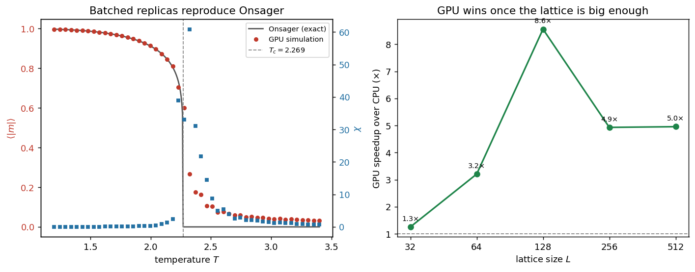

The GPU sustains roughly 640 million spin-updates per second and a peak 8.6× speedup over the multithreaded CPU. The caveat is the small-lattice end: at $L=32$ the GPU is barely ahead, because kernel-launch and dispatch overhead dominates when there isn't enough work to fill the device. The speedup only pays off once the lattice is big enough to saturate it — and past $L=128$ it eases back toward $5\times$ as the problem becomes memory-bandwidth bound rather than compute bound. Knowing where the GPU wins is the point of running the sweep, not just quoting the peak.

Extensions

The batched-lattice pattern generalizes well beyond a speedup demo.

1. Parallel tempering along the batch. The replicas are already at different temperatures — periodically propose swaps between adjacent ones. You get replica-exchange Monte Carlo almost for free, and it beats single-temperature sampling through the critical slowdown.
2. A real CUDA kernel. PyTorch's op-by-op dispatch leaves throughput on the table. Write the checkerboard update as one fused CUDA kernel with the spins in shared memory and compare against the framework version — the gap is the framework overhead this benchmark is paying.
3. Cluster moves on the GPU. Wolff and Swendsen–Wang beat single-spin dynamics near $T_c$, but cluster-finding is inherently sequential. Implement the parallel label-propagation version and measure whether the better algorithm or the better hardware wins.
4. Push the batch. Throughput scales with occupancy — grow $B$ until the device saturates and plot spin-updates/s vs batch size to find the knee.
5. Precision sweep. Spins are $\pm 1$; do the accept/reject in float16 and find where, if anywhere, the reduced precision moves $T_c$.