“Know how to solve every problem that has been solved.” “What I cannot create, I do not understand.” — Richard Feynman

Project: 2D Ising Model

Projects

The goal. Build a Metropolis Monte Carlo simulation of the 2D Ising model on a 32×32 periodic lattice, measure the magnetization, energy, specific heat, and susceptibility across the phase transition, and locate the critical temperature within a few percent of Onsager's exact result. The prototype is one self-contained Python file (~60 lines) and runs in about 30 seconds on a laptop. The extensions take it from "I copied a textbook simulation" to "I built a working tool for studying phase transitions."

The math

Spins $s_{i} \in {- 1, + 1}$ sit on the sites of an $L \times L$ lattice. Nearest neighbors interact ferromagnetically:

H = - J ⟨ i, j ⟩ \sum s_{i} s_{j},

with periodic boundary conditions and $J = 1$ . We sample configurations from the Boltzmann distribution $P ({s}) \propto e^{- H / T}$ using the Metropolis-Hastings algorithm: propose a single spin flip, accept it with probability $min (1, e^{- Δ E / T})$ .

Onsager (1944) solved this exactly. The critical temperature is

T_{c} = \frac{2}{ln ( 1 + 2 )} \approx 2.2692 J / k_{B} .

Below $T_{c}$ , the spontaneous magnetization follows

m (T) = [1 - sinh^{- 4} (\frac{2 J}{T})]^{1/8} .

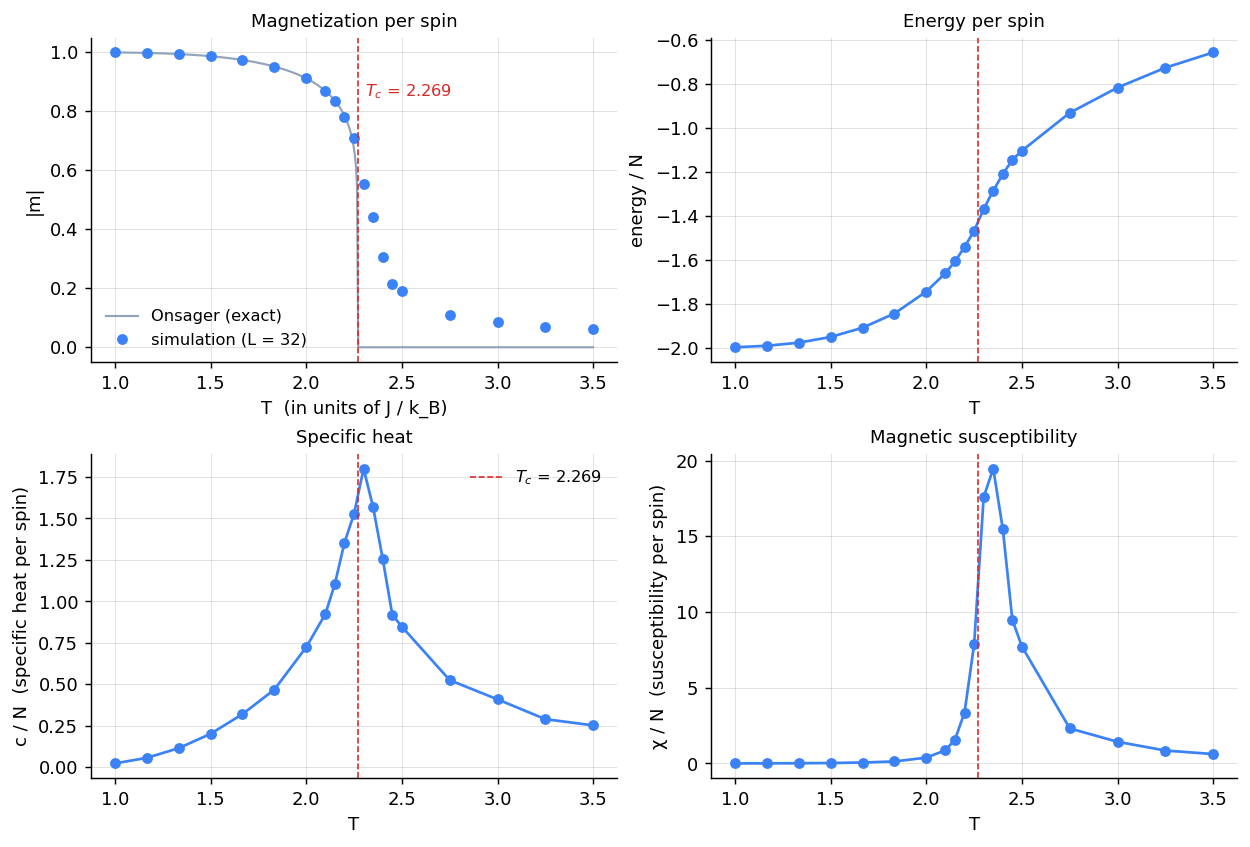
Above $T_{c}$ , $m = 0$ in the thermodynamic limit. In a finite system, $m$ never sharply discontinues — instead, $⟨ ∣ M ∣ ⟩ / N$ rounds smoothly across $T_{c}$ , and the specific heat and susceptibility peak at a finite-size–shifted temperature slightly above the true $T_{c}$ . We measure four observables:

$e = ⟨ H ⟩ / N$ — energy per spin
$∣ m ∣ = ⟨ ∣ M ∣ ⟩ / N$ — order-parameter magnitude (using $∣ M ∣$ avoids cancellation when the simulation flips sign)
$c = (⟨ E^{2} ⟩ - ⟨ E ⟩^{2}) / (N T^{2})$ — specific heat per spin (fluctuation-dissipation form)
$χ = (⟨ M^{2} ⟩ - ⟨ ∣ M ∣ ⟩^{2}) / (NT)$ — magnetic susceptibility per spin

The prototype

A vectorized checkerboard Metropolis sweep. Color the lattice like a chessboard. Every "black" site has only "white" neighbors, so all black sites can be updated in parallel (no races) and then all white sites. One sweep becomes two vectorized array operations instead of $L^{2}$ Python loop iterations — about two orders of magnitude faster.

"""
2D Ising model on an L x L periodic lattice, vectorized checkerboard
Metropolis sweep.

Hamiltonian:  H = -J * sum_<i,j> s_i s_j   with J = 1, k_B = 1.

Why checkerboard:
    A site's update depends only on its four nearest neighbors. Color the
    lattice like a chessboard; every "black" site sees only "white" neighbors.
    All black sites can be flipped in parallel without races, then all white
    sites. One sweep = 2 vectorized array operations instead of L*L Python
    iterations. Roughly two orders of magnitude faster than the naive loop.
"""
import numpy as np

J  = 1.0
TC = 2.0 / np.log(1.0 + np.sqrt(2.0))       # Onsager 1944

def checkerboard_step(s, T, mask_black, rng):
    """One full sweep: update black sublattice, then white sublattice."""
    beta = 1.0 / T
    for is_black in (True, False):
        mask = mask_black if is_black else ~mask_black
        nbr  = (np.roll(s,  1, axis=0) + np.roll(s, -1, axis=0)
              + np.roll(s,  1, axis=1) + np.roll(s, -1, axis=1))
        dE   = 2 * J * s * nbr
        rand = rng.random(s.shape)
        flip = ((dE <= 0) | (rand < np.exp(-beta * dE))) & mask
        s[flip] = -s[flip]


def run_at_T(T, L=32, n_sweeps=4000, n_eq=1000, seed=0):
    rng = np.random.default_rng(seed)
    s   = rng.choice([-1, 1], size=(L, L)).astype(np.int8)
    ii, jj = np.indices((L, L))
    mask_black = ((ii + jj) % 2 == 0)

    for _ in range(n_eq):
        checkerboard_step(s, T, mask_black, rng)

    E = np.empty(n_sweeps); M = np.empty(n_sweeps)
    for k in range(n_sweeps):
        checkerboard_step(s, T, mask_black, rng)
        nn_right = np.roll(s, -1, axis=1)
        nn_down  = np.roll(s, -1, axis=0)
        E[k] = -J * np.sum(s * nn_right + s * nn_down)
        M[k] = s.sum()

    N = L * L
    return dict(
        T=T,
        e=E.mean() / N,
        m=np.abs(M).mean() / N,
        c=E.var() / (N * T * T),
        chi=(np.mean(M ** 2) - np.abs(M).mean() ** 2) / (N * T),
        final=s.copy(),
    )


def onsager_m(T, Tc=TC):
    if T >= Tc: return 0.0
    return (1.0 - np.sinh(2.0 / T) ** -4) ** (1.0 / 8.0)


# ---- Sweep T across the transition --------------------------------------
print(f"Onsager Tc = 2 / ln(1 + sqrt(2)) = {TC:.4f}")
Ts = np.concatenate([np.linspace(1.0, 2.0, 7),
                     np.linspace(2.10, 2.45, 8),
                     np.linspace(2.5, 3.5, 5)])
print(f"{'T':>6}  {'e/N':>10}  {'|m|':>8}  {'c/N':>8}  "
      f"{'chi/N':>8}  {'m_onsager':>10}")
print("-" * 65)
for T in Ts:
    r = run_at_T(T, L=32, n_sweeps=4000, n_eq=1000, seed=0)
    print(f"{T:6.3f}  {r['e']:10.4f}  {r['m']:8.4f}  {r['c']:8.4f}  "
          f"{r['chi']:8.3f}  {onsager_m(T):10.4f}")

Running across 20 temperatures from $T = 1.0$ to $3.5$ :

Onsager Tc = 2 / ln(1 + sqrt(2)) = 2.2692
     T         e/N       |m|       c/N     chi/N   m_onsager
-----------------------------------------------------------------
 1.000     -1.9973    0.9993    0.0225     0.002      0.9993
 1.167     -1.9905    0.9975    0.0559     0.005      0.9976
 1.333     -1.9765    0.9937    0.1144     0.012      0.9938
 1.500     -1.9505    0.9864    0.2008     0.027      0.9865
 1.667     -1.9086    0.9734    0.3196     0.061      0.9736
 1.833     -1.8441    0.9515    0.4675     0.130      0.9514
 2.000     -1.7442    0.9109    0.7236     0.381      0.9113
 2.100     -1.6605    0.8675    0.9232     0.872      0.8687
 2.150     -1.6076    0.8349    1.1059     1.576      0.8357
 2.200     -1.5421    0.7815    1.3546     3.363      0.7848
 2.250     -1.4681    0.7079    1.5278     7.857      0.6719
 2.300     -1.3692    0.5518    1.8012    17.594      0.0000   ← peak c
 2.350     -1.2858    0.4420    1.5669    19.476      0.0000   ← peak chi
 2.400     -1.2112    0.3073    1.2553    15.479      0.0000
 2.450     -1.1456    0.2137    0.9189     9.476      0.0000
 2.500     -1.1046    0.1923    0.8472     7.718      0.0000
 2.750     -0.9322    0.1083    0.5247     2.311      0.0000
 3.000     -0.8177    0.0851    0.4088     1.428      0.0000
 3.250     -0.7275    0.0698    0.2892     0.851      0.0000
 3.500     -0.6580    0.0619    0.2519     0.618      0.0000

The first four temperatures track Onsager's analytic $m (T)$ to four decimal places. The specific heat peaks at $T \approx 2.30$ , the susceptibility at $T \approx 2.35$ — both are finite-size–shifted estimates of the true $T_{c} = 2.269$ . The shift is $\sim 1/ L$ , so at $L = 32$ you're already within a few percent without doing anything fancy.

The output

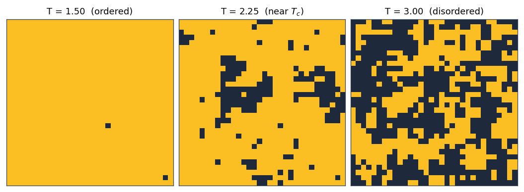
Four panels of Ising observables vs temperature on a 32x32 lattice. Magnetization curve drops sharply from 1 to 0 across T_c marked at 2.269. Simulation points lie on top of the Onsager analytic curve below T_c. Energy curve rises smoothly through the transition. Specific heat shows a peak at T = 2.30. Susceptibility shows a sharp peak at T = 2.35.

Snapshots of three representative configurations show what's happening at the microscopic level. Below $T_{c}$ , almost every spin aligns. Near $T_{c}$ , clusters of every size coexist (the system is scale-invariant). Above $T_{c}$ , the configuration looks like uncorrelated noise.

Three 32x32 lattice snapshots. T = 1.50 (ordered): nearly all spins are the same color, with a few small inclusions. T = 2.27 (near critical): nested clusters of both colors at every size scale, no single domain. T = 3.00 (disordered): salt-and-pepper noise, no long-range structure.

Extensions

Each of these takes the prototype and turns it into a real research-flavored study. Pick one, write the code, run it, plot the result.

Susceptibility critical exponent. Above $T_{c}$ , susceptibility diverges as $χ \sim ∣ T - T_{c} ∣^{- γ}$ with $γ = 7/4$ in 2D. Fit $lo g χ$ vs $lo g ∣ T - T_{c} ∣$ in the range $T \in [2.4, 3.0]$ , away from finite-size rounding. Verify the slope is close to $- 1.75$ . (The fit will be imperfect at $L = 32$ ; that's the point of the next exercise.)
Finite-size scaling and a sharper $T_{c}$ estimate. Run at $L = 8, 16, 32, 64$ . Plot the Binder cumulant $U_{4} = 1 - ⟨ M^{4} ⟩ / (3 ⟨ M^{2} ⟩^{2})$ vs $T$ for each $L$ . The curves cross at the true $T_{c}$ (the location where $U_{4}$ is $L$ -independent). This is the textbook way to extract $T_{c}$ from finite-system simulations.
Wolff cluster algorithm. Near $T_{c}$ the single-flip Metropolis dynamics slows critically — autocorrelation times grow like $τ \sim L^{z}$ with $z \approx 2.17$ for the 2D Metropolis algorithm. Implement Wolff's cluster algorithm: pick a random seed site, grow a cluster by adding aligned neighbors with probability $p = 1 - e^{- 2 J / T}$ , flip the whole cluster. Wolff has $z \approx 0.25$ — orders of magnitude faster decorrelation at $T_{c}$ .
Spatial correlations at $T_{c}$ . Compute $g (r) = ⟨ s_{0} s_{r} ⟩$ as a function of distance. Below $T_{c}$ , $g (r) \to m^{2}$ (long-range order). Above $T_{c}$ , $g (r) \sim e^{- r / ξ}$ with finite correlation length $ξ$ . At $T_{c}$ , $g (r) \sim r^{- η}$ with $η = 1/4$ . Verify the algebraic decay on a log-log plot at $T = T_{c}$ .
External magnetic field. Add a Zeeman term $- h \sum_{i} s_{i}$ to the Hamiltonian. Map out $m (h, T)$ for fixed $T < T_{c}$ and observe the hysteresis loop as you sweep $h$ from $- 2$ to $+ 2$ at a rate that's slow compared to $τ$ but fast compared to the rare flips between metastable states. (The coercive field decreases as $T \to T_{c}$ .)
3D Ising on a cube. Generalize the prototype to a cubic lattice. $T_{c} \approx 4.5115$ in 3D, no closed form (Onsager only solved 2D). Specific-heat peak should land near there. The 3D exponents are different from 2D ( $γ \approx 1.24$ , $β \approx 0.326$ , $η \approx 0.036$ ) — verify them and you've reproduced the canonical results of computational statistical mechanics.
Live visualization. Wrap the per-sweep update in a matplotlib animation: show the lattice updating in real time at a chosen $T$ . The contrast between ordered, critical, and disordered regimes is much more vivid when you can see the dynamics. Tune the sweep rate so the cluster structure at $T_{c}$ is visible by eye.

References

Onsager, L. (1944). "Crystal statistics. I. A two-dimensional model with an order-disorder transition." Phys. Rev., 65, 117–149. (The exact solution.)
Newman, M. E. J. & Barkema, G. T. (1999). Monte Carlo Methods in Statistical Physics, Oxford. (Standard reference for Metropolis, Wolff, finite-size scaling, and the technique behind every extension on this page.)
Wolff, U. (1989). "Collective Monte Carlo updating for spin systems." Phys. Rev. Lett., 62, 361. (The cluster algorithm.)
Binder, K. (1981). "Finite size scaling analysis of Ising model block distribution functions." Z. Phys. B, 43, 119–140. (The cumulant trick for extracting $T_{c}$ from small lattices.)

Related on this site

The Ising model concept page covers the theory the simulation is implementing. MCMC from scratch is the Metropolis-Hastings algorithm without the lattice. The Hartree-Fock SCF loop is a different kind of fixed-point iteration on a different physical system.