An Orchestrator: AI-Feynman Decomposition Meets a Solver Portfolio

Three engines elsewhere on this site attack symbolic regression by three different routes — a genetic search over expression trees, SISSO's compressed-sensing sweep of a feature space, and a trained transformer that generates formulas from a learned prior. All three share one weakness: they degrade as the number of variables grows, because the tree space, the feature count, and the sequence length all explode with dimension. AI-Feynman's contribution is a way to dodge that explosion — use the structure of physics to break a many-variable law into one-variable pieces. This page wires the two ideas together into a single method: AI-Feynman's decomposition on the outside, a portfolio of all three solvers on the inside. The decomposition manufactures exactly the easy case — a single variable — that each engine is strongest on, and the portfolio lets the best tool win each piece.

Separability turns n variables into n problems

The reduction AI-Feynman leans on hardest is separability. Many laws factor: a force that is a product of a charge term and a distance term, an energy that is a sum of a kinetic and a potential piece. If $f(x,y)=g(x)\cdot h(y)$ or $f(x,y)=g(x)+h(y)$, then the two variables never actually interact, and finding $f$ is really two independent one-variable searches. The trick is detecting this from data alone. Fit a smooth surrogate to the scattered points so you can probe the function anywhere, then hold every variable but one fixed at a base point and read off the resulting one-dimensional profile along each axis. If those profiles add back up to the data, the law is additively separable; if they multiply back, it is multiplicatively separable (which is just additive separability of $\log f$). Whichever reconstruction matches is both the diagnosis and the decomposition — the profiles are the one-variable subproblems.

def surrogate(X, y):                 # 1. a smooth stand-in we can probe ANYWHERE
    return RBFInterpolator(X, y, kernel='thin_plate_spline')

def detect(rbf, X, x0):              # 2. hold all but one variable fixed at a base point x0
    # profile_i(t) = f(x0 with coordinate i replaced by t)  -- a 1-D slice of the surface
    profs = [rbf(vary_only(i, x0)) for i in range(n_vars)]
    r2_add = affine_fit(sum(profs),  y)     # do the slices ADD back to the data?
    r2_mul = scale_fit(prod(profs),  y)     # or MULTIPLY back? (mult = additive in log)
    return 'add' if r2_add > r2_mul else 'mul'     # whichever reconstructs f is the structure

def portfolio(x, y):                # 3. every 1-D leaf -> all three engines COMPETE
    cands = [gp_solve(x, y),        #    genetic programming
             sisso_solve(x, y),     #    SISSO
             symgpt_solve(x, y)]    #    the trained transformer
    return simplest_within(cands, tol=0.005)       # keep the cleanest near-best formula

That last function is where the four methods become one. Each one-variable leaf is handed to a portfolio — the genetic search, SISSO, and the transformer all attempt it, and the orchestrator keeps the simplest formula that comes within a whisker of the best fit. This is the piece plain AI-Feynman does not have: it uses a polynomial fit or a brute-force table at its leaves, whereas here three genuinely different symbolic engines compete for each one. And it is the only setting in which the transformer can even play — it was trained on a single variable, so the decomposition is what hands it a problem it can solve. The reductions build the transformer's home turf.

Decompose-and-conquer beats the monolith

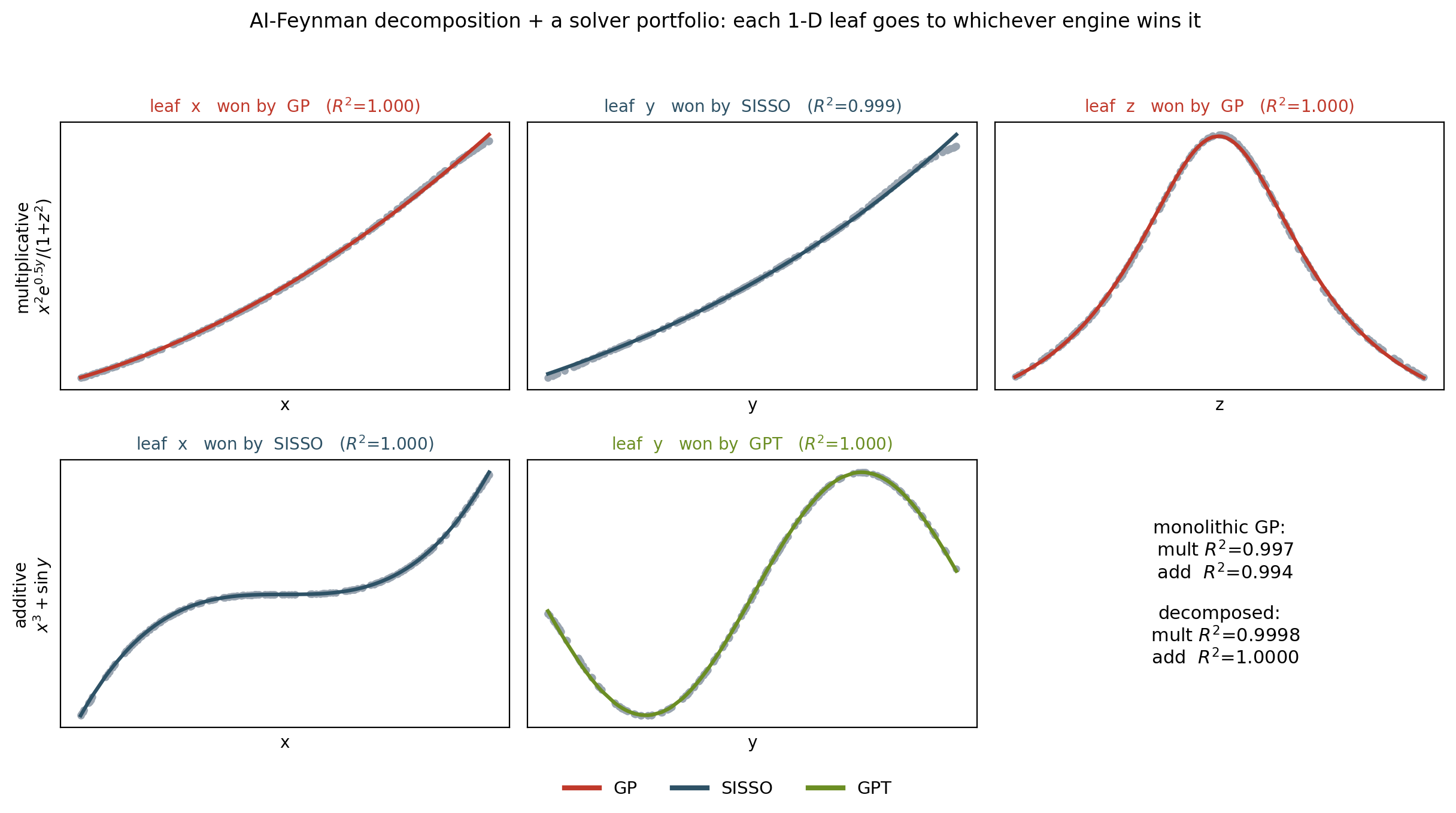
Two targets show it working. The first is a three-variable multiplicative law, $f=x^2{e}^{0.5y}/(1+z^2)$; the second an additive one, $f=x^3+\sin y$. Handed all variables at once, the monolithic genetic search gets close but not exact and returns a sprawling expression, while SISSO stalls badly on the product ($R^2=0.89$). The orchestrator detects the separability, splits each into one-variable leaves, and lets the portfolio settle them:

=== f = x^2 * exp(0.5 y) / (1 + z^2)      [3 variables] ===
  monolithic baseline (all variables at once):   GP R2 = 0.997    SISSO R2 = 0.893
  separability detected:  MULTIPLICATIVE
    leaf x:   GP 1.000   SISSO 1.000   GPT  1.000    ->  GP     x^2
    leaf y:   GP 0.999   SISSO 0.999   GPT  0.319    ->  SISSO  sqrt(exp(y)) = exp(0.5 y)
    leaf z:   GP 1.000   SISSO 0.977   GPT -1.223    ->  GP     1 / (1 + z^2)
  recombine (product) + one global fit:           R2 = 0.99984

=== f = x^3 + sin(y)                      [2 variables, additive] ===
  monolithic baseline:                            GP R2 = 0.994    SISSO R2 = 0.984
  separability detected:  ADDITIVE
    leaf x:   GP 1.000   SISSO 1.000   GPT  0.996    ->  SISSO  x^3
    leaf y:   GP 0.909   SISSO 0.845   GPT  1.000    ->  GPT    sin(y)
  recombine (sum) + one global fit:               R2 = 1.00000

The division of labor is the point. On the multiplicative law the genetic search claims the polynomial and the Lorentzian leaves while SISSO recognizes the exponential (as $\sqrt{e^y}=e^{0.5y}$, a single constructed feature); on the additive law SISSO takes the cubic and the transformer — in its trained one-variable regime — nails the sine that the other two only approximate. No single engine wins every leaf, and that is exactly why running all three beats committing to one. Recombine the leaf formulas with a product or a sum, fit one global constant, and the three-variable law lands at $R^2=0.9998$ and the additive one at $R^2=1.00000$ — from a data-only start, with an interpretable factored formula rather than the monolith's tangle.

What makes it hard, and what real AI-Feynman adds

• The surrogate is the weak link. Every separability test runs on the fitted interpolant, not the true function, so its accuracy caps everything downstream. A radial-basis fit is fine for a few variables and a hundred-odd points; real AI-Feynman trains a neural network on far more data precisely because the reductions are only as trustworthy as the surface they probe.
• Separability is one reduction among many. AI-Feynman also tests for translational and scaling symmetry, for compositionality ($f=g(h(x,y))$), and — before anything else — uses dimensional analysis to shed variables outright. Each is another way to shrink the problem; this page implements the two separability tests, which already carry a large fraction of textbook physics.
• The transformer is boxed in by its training. SymGPT recovers a leaf only if that leaf resembles its training distribution — one variable, a known operator set, values in range. Push a leaf outside that box and it fails, which is why it must sit inside a portfolio with two engines that search rather than recall.
• Recombination hides a subtlety. Each profile carries a base-point constant along for the ride, so the leaf formulas are correct only up to an overall factor or offset. One global least-squares fit at the end absorbs those constants — the reason the method reports the shape exactly but leaves the single overall calibration to the recombination step.

The point, for a computational scientist

A real law from a simulation rarely depends on one variable — an adsorption energy varies with coverage and strain and composition at once, a rate with temperature and pressure and concentration. That is the regime where every single-strategy symbolic regressor struggles and where this composition earns its keep: use physics to argue the law separates, and a hard multivariable discovery collapses into a handful of one-variable ones, each dispatched to whichever of the three engines handles it best. It is the capstone of the symbolic-regression canon on this site — not a fourth method, but the argument that the three are complementary tools and that the right move on a hard problem is to reach for a decomposition and then let them compete.

Reproduce it

scripts/gen_hybrid_sr.py is the orchestrator: an RBF surrogate, the additive and multiplicative separability tests, a portfolio leaf-solver that calls the genetic-programming engine, SISSO, and the trained SymGPT model in turn, and the recombination with a final global fit. It imports all three engines directly from the rest of this site — nothing is reimplemented — and recovers $x^2{e}^{0.5y}/(1+z^2)$ and $x^3+\sin y$ from data alone, reporting which engine won each leaf. The decomposition idea is Udrescu and Tegmark, Sci. Adv. 6, eaay2631 (2020); the portfolio of three from-scratch solvers is what this site adds to it.