“Know how to solve every problem that has been solved.” “What I cannot create, I do not understand.” — Richard Feynman

SISSO: Symbolic Regression as Compressed Sensing

Machine Learning

The genetic-programming approach to symbolic regression searches the space of expression trees directly, breeding formulas that fit. SISSO refuses to search at all. It comes from materials science — where the question is often which combination of a material's tabulated properties predicts whether it is a metal or an insulator — and it answers by brute construction followed by compressed sensing. Take a handful of primary variables, apply an operator set to them over and over to manufacture an astronomical list of candidate features, and then use a correlation screen and an $ℓ_{0}$ selection to pick out the two or three that a simple linear model needs. The name is the recipe: Sure Independence Screening and Sparsifying Operator. This page builds it from scratch and watches it pull Coulomb's law — constant and all — out of a feature space of twelve thousand candidates.

Build a universe of features, then screen it

A "feature" here is any analytic expression in the primary variables: $r$ , then $r^{2}$ , then $q_{1} q_{2}$ , then $(q_{1} q_{2}) / r^{2}$ , and on outward. SISSO builds them in rungs. Rung zero is the raw variables; each further rung applies every operator in the set — arithmetic, squares, roots, $exp$ , $lo g$ , absolute values — to everything built so far. Two rungs of a seven-operator set on four variables already gives around twelve thousand distinct features; three rungs reaches the billions, which is where the real code lives. This is the opposite of the tree search: instead of cleverly walking a giant space, SISSO enumerates it and then throws almost all of it away.

Throwing it away is the screening step, and it is embarrassingly simple: standardize every candidate feature, take its correlation with the target, and keep the few dozen with the largest magnitude. That is Sure Independence Screening — a name borrowed from the statistics of high-dimensional regression, where it comes with a guarantee that the truly relevant variables survive the cut with high probability. What survives is a small, hand-inspectable shortlist. The Sparsifying Operator then does the actual model selection: for a one-dimensional descriptor it takes the single best feature; for higher dimensions it searches subsets of the shortlist for the smallest set whose linear combination fits the data. Searching for the smallest good-enough subset is $ℓ_{0}$ regularization — the pure form of "use as few features as possible," and the reason the output is a short formula instead of a dense fit over thousands of terms.

# A feature = (symbolic name, values over samples, complexity).  Primaries: complexity 0.
UNARY  = [('({})^2', sq), ('sqrt({})', psqrt), ('1/({})', pinv),
          ('exp({})', pexp), ('log({})', plog), ('|{}|', abs)]
BINARY = [('({} + {})', add, SYM), ('({} - {})', sub), ('({} * {})', mul, SYM),
          ('({} / {})', pdiv),      ('|{} - {}|', absdiff, SYM)]

def build_space(feats, rungs=2):            # 1. CONSTRUCT
    for _ in range(rungs):                  # each rung applies every operator once more
        for f in feats:        emit unary(f)
        for a, b in pairs(feats):
            emit binary(a, b)               # non-symmetric ops (/, -) -> BOTH orderings
    return dedup(feats)                     # a few thousand candidate analytic features

def sis(space, y, keep=40):                 # 2. SCREEN -- Sure Independence Screening
    corr = abs(standardize(space).T @ standardize(y))   # |correlation| with the target
    return top_k(space, corr, keep)         # the only features worth considering

def sparsify(screened, y, max_dim=2):       # 3. SELECT -- Sparsifying Operator (l0)
    for D in 1 .. max_dim:                   # smallest set of features whose LINEAR
        best[D] = argmax over D-subsets:     #   combination reproduces the target
                    r2(least_squares(subset, y))
    return best                             # a compact, readable descriptor

One subtlety decides whether it works. The non-symmetric operators — $\div$ and subtraction — have to be applied in both orderings when features are combined, or half the space never gets built: manufacture $r^{2} / (q_{1} q_{2})$ but never $(q_{1} q_{2}) / r^{2}$ , and Coulomb's law is simply not in your universe of features, so no amount of screening can find it. And because the target feature might sit at complexity three while thousands of simpler features crowd beneath it, the construction must keep the whole rung, not a truncated sample of it — the screen, not an arbitrary size cap, is what does the discarding.

Coulomb's law from a feature soup

A three-stage horizontal funnel. The top bar, 12,758 constructed features, is very wide; the middle bar, the top 40 kept by screening, is much shorter; the bottom bar, the single-feature law selected, is tiny.

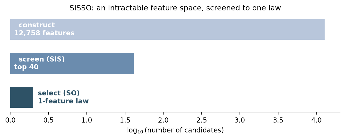
Give the engine four primaries — two charges $q_{1}, q_{2}$ , a distance $r$ , and one irrelevant decoy variable — and the target $F = k q_{1} q_{2} / r^{2}$ , with no hint of the form. It constructs 12,758 features, screens to 40, and selects:

=== 1D recovery:  Coulomb   F = k q1 q2 / r^2     (primaries: q1, q2, r, + a decoy) ===
  feature space built: 12758 candidates
  D=1:   R2 = 1.000000    F =  +8.99 * [ (q1*q2) / r^2 ]      <-- exact law AND the constant k
  D=2:   R2 = 1.000000    ... same descriptor + a redundant second term

=== 1D recovery:  pendulum  T = 2*pi*sqrt(L/g)               (primaries: L, g) ===
  feature space built: 980 candidates
  D=1:   R2 = 1.000000    T =  +6.283 * [ sqrt(L/g) ]         (6.283 = 2*pi)

=== 2D recovery:  y = 3(q1 q2) + 5/r      (one feature cannot do it) ===
  D=1:   R2 = 0.999812    y = +3.00 * [ (q1*q2) - sqrt(r) ]   best single feature: close, not exact
  D=2:   R2 = 1.000000    y = +5*[ 1/r + q1*q2 ] - 2*[ q1*q2 ]   two features -> 5/r + 3 q1 q2

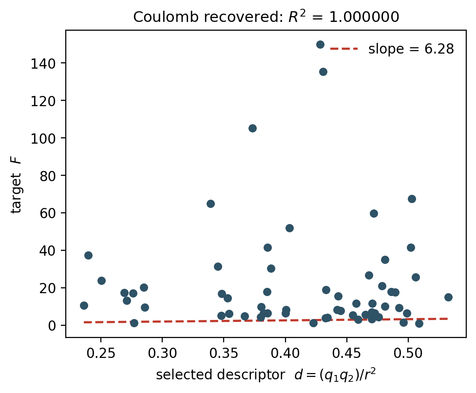
Scatter plot of the target force F against the selected descriptor (q1 q2 over r squared). Every point lies exactly on a straight line through the origin with slope 8.99.

The one-dimensional descriptor is $(q_{1} q_{2}) / r^{2}$ with $R^{2} = 1.000000$ , and the fitted coefficient is $8.99$ — not just the right shape but Coulomb's constant $k = 8.99 \times 1 0^{9}$ in the units of the data. The decoy variable never appears; its correlations were too weak to survive the screen. Compare this to the genetic-programming route to the same kind of answer: there is no population, no mutation, no random seed, and no run-to-run variability. The feature was either constructed or it was not, and if it was, the correlation screen finds it every time. SISSO is deterministic symbolic regression, and that determinism is exactly why materials scientists trust it to report a descriptor they will publish.

When one feature is not enough

Two more targets show the dimensional ladder. A pendulum's period $T = 2 π L / g$ falls out at one dimension — the engine builds $L / g$ and fits the coefficient to $6.283 = 2 π$ . But a genuinely two-term law, $y = 3 q_{1} q_{2} + 5/ r$ , cannot be a single constructed feature times a constant, and the front says so: the best one-dimensional descriptor reaches only $R^{2} = 0.9998$ before stalling, and the search has to grow to two features to hit $R^{2} = 1$ . That is the sparsifying operator earning its name — it reports the smallest dimension that suffices, so the jump from "excellent one-feature fit" to "exact at two features" is the tell that the physics genuinely has two independent contributions, not one.

Sharper screens: distance correlation and bootstrap stability

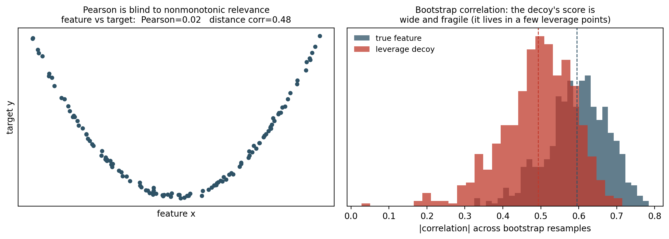
The whole method leans on the screen, and the screen leans on one number — the correlation between each feature and the target. Pearson correlation, the default choice, has two blind spots worth patching. It sees only linear association, so a feature that is genuinely relevant but related nonmonotonically — through an even or oscillatory link — scores near zero and is thrown away. Distance correlation (Székely–Rizzo–Bakirov 2007) instead measures any statistical dependence and is zero only under true independence; on a feature that drives the target through a parabola it reads $0.48$ where Pearson reads $0.02$ and would screen it out.

Left: a scatter of target against feature forming a clean parabola, annotated Pearson 0.02, distance correlation 0.48. Right: histograms of each feature's correlation across bootstrap resamples — the true feature's is high and tight, the leverage decoy's is lower and much wider.

The second blind spot: a one-shot correlation can be high by accident. With few samples, a decoy that happens to line up on this particular draw — usually because of a handful of high-leverage points — can steal a screening slot from a real feature. Resampling the data a few hundred times exposes it. A genuine feature's correlation stays high and tight across resamples; a leverage-driven one swings wildly, collapsing whenever a resample drops its few load-bearing points (a decoy at one-shot $∣ r ∣ = 0.50$ falls to $0.04$ once its five leverage points are removed). Ranking by a lower confidence bound — mean minus spread — rather than the raw score demotes the impostor. Both are one-line swaps for the correlation call (sis(..., metric='dcor') selects the first), and both harden the one step everything downstream depends on.

What makes it hard, and what the real code adds

The feature space explodes. Each rung multiplies the count by the operator set size squared; the reference Fortran routinely constructs $1 0^{10}$ candidates and screens them in a distributed sweep. The whole method is an exercise in making that explosion survivable — the screen is the pressure valve.
Dimensional analysis is a free scythe. Real SISSO tracks units and refuses to add a length to an energy or take the logarithm of a dimensioned quantity. That single rule deletes most of the feature space before it is scored — the teaching version here skips it, which is why the decoy has to be beaten on correlation alone.
The $ℓ_{0}$ select is combinatorial. Exhaustively checking every $D$ -subset is only tractable because the screen already shrank the pool to a few dozen; grow the descriptor dimension and the subset search is where the cost goes. Production code uses the screened residuals to grow the descriptor greedily rather than searching all subsets at once.
It classifies, too. Swap the linear least-squares fit for a convex-hull overlap criterion and the same construct–screen–select loop finds descriptors that separate classes — metal versus insulator, stable versus unstable structure — which is the application that made SISSO famous.

The point, for a computational scientist

SISSO's home is exactly the table a simulation campaign produces: one row per material, columns of cheap computed or tabulated properties — atomic radii, electronegativities, ionization energies — and a target you care about, a band gap or an adsorption energy or a formation enthalpy. It was built to answer "what simple combination of these predicts the property," and it answers with a descriptor a chemist can read and reason about, not a black box. That makes it the deterministic counterpart to the evolutionary and learned engines elsewhere in this canon: same goal — a formula from a data table — reached by compressed sensing instead of search. When a DFT study on this site ends with a table and the question "what law do these numbers obey," this is one of the three tools it hands the table to.

Know this cold

SISSO: know this cold

Unlike genetic programming, SISSO has no random seed: the feature space is fixed, the screen is a deterministic sort, and the selection is an exhaustive best-subset search, so it returns the same descriptor every run. This reproducibility is why materials scientists publish SISSO descriptors.
where this comes from →
Non-symmetric operators ( $\div$ , $-$ ) must be applied in both orderings when constructing features, or half the space is never built. If $(q_{1} q_{2}) / r^{2}$ is never constructed, no screen can find Coulomb's law; the failure is silent because a plausible high-correlation feature is returned instead.
where this comes from →
Sure Independence Screening ranks every candidate feature by the magnitude of its correlation with the target and keeps only the top few dozen; it is dimensionality reduction with a high-probability guarantee that the truly relevant features survive.
where this comes from →
The Sparsifying Operator is $ℓ_{0}$ regularization: for each descriptor dimension $D$ it finds the $D$ -feature subset whose linear least-squares fit is best, reporting the smallest $D$ that suffices. The jump from a near-perfect 1D fit to an exact 2D fit signals two independent physical contributions.
where this comes from →
SISSO has three deterministic steps: construct a huge feature space by applying an operator set in rungs, Sure Independence Screening (SIS) to keep the top features by $∣$ correlation $∣$ with the target, then a Sparsifying Operator (SO) that $ℓ_{0}$ -selects the smallest feature subset whose linear combination fits.
where this comes from →

Try First

Each prompt asks a checkable question about the working code or math above — predict an output, derive a sign, state an invariant, find a bug. Commit to an answer before clicking "reveal." That commitment is the whole point: if your answer matched, you understand the piece you were looking at; if it didn't, that's the part worth re-reading.

predict

The engine builds

(q_{1} q_{2}) / r^{2}

and recovers Coulomb's law. If a bug made the binary operators apply in only one ordering — so

a / b

is built but never

b / a

— what would the Pareto output look like, and why is this failure so easy to miss?

why does this work

Genetic programming and SISSO both return an interpretable formula. Why might a materials scientist reach for SISSO specifically, over the evolutionary search, even when both would find the answer?

Reproduce it

scripts/gen_sisso.py is the whole method — rung-based feature construction, the correlation screen, and the exhaustive $ℓ_{0}$ descriptor search — in about two hundred lines over NumPy alone. It recovers Coulomb's law with its constant from a 12,758-feature space ( $R^{2} = 1.000000$ ), the pendulum period at one dimension, and a two-term target at two. Add a primary variable, extend to a third rung, or feed it your own property table and read off the descriptor. The method is Ouyang, Curtarolo, Ahmetcik, Scheffler, and Ghiringhelli, Phys. Rev. Materials 2, 083802 (2018); this is an independent teaching reimplementation of their idea.