Symbolic Regression: Rediscovering Physical Laws from Data

Ordinary regression fits the parameters of a form you already chose: you decide the model is a line, or a Gaussian, or a power law, and least squares hands you the coefficients. Symbolic regression asks the harder question — what is the form? Given a table of numbers, it searches the space of algebraic expressions themselves, built from $+,-,\times ,÷,\sqrt{},\dots$ and the input variables, and returns a formula. Kepler spent years staring at Tycho Brahe's orbital tables before he saw that the period squared goes as the radius cubed. This page builds a symbolic-regression engine from scratch — a real genetic-programming search, no libraries — hands it the same eight planets, and watches it recover Kepler's third law in a few seconds of evolution.

Searching the space of formulas

Represent every candidate law as an expression tree: internal nodes are operators, leaves are variables or constants. The space of such trees is the space of all formulas, and it is astronomically large — which is exactly why you search it the way evolution searches genotypes. Start with a population of random trees. Score each by how well it fits the data. Breed the good ones: crossover splices a subtree from one formula into another; mutation perturbs a node. Repeat. Good structure — a ​ here, a product there — survives and spreads because the trees that carry it fit better. It is curve-fitting where the curve's shape is the thing under selection.

One decision makes symbolic regression work instead of embarrassing itself. Left to minimize error alone, the search will grow a monster: a tree with forty nodes can thread every data point including the noise, and it will report a "law" that is really a memorized table. The cure is to refuse to optimize accuracy in isolation and instead track the Pareto front — the best-fitting expression at each level of complexity — and then read off the one at the elbow, where accuracy stops improving and complexity keeps climbing. That elbow is where a law lives: the simplest expression that explains the data, and not one node more.

# Expression trees:  ['op', child, ...]  or  ('var', i)  or  ('const', c)
# Protected operators so a bad subtree just scores poorly instead of crashing.
OPS = {'add': (2, add), 'sub': (2, sub), 'mul': (2, mul), 'div': (2, pdiv),
       'sqrt': (1, psqrt), 'sq': (1, square), 'log': (1, plog)}

def evaluate(tree, x):                       # x = the input variables of one sample
    if tree[0] == 'var':   return x[tree[1]]
    if tree[0] == 'const': return tree[1]
    return OPS[tree[0]][1](*[evaluate(c, x) for c in tree[1:]])

def fit_and_score(tree, X, y):               # fit  a*expr + b  by least squares
    p = predict(tree, X)                     # -> the shape is discovered, the
    A = np.vstack([p, np.ones_like(p)]).T    #    two constants are fit linearly
    (scale, off), *_ = np.linalg.lstsq(A, y, rcond=None)
    return np.sqrt(np.mean((y - (scale * p + off)) ** 2))     # RMSE

# Evolve, and keep the BEST expression seen at each complexity -> the Pareto front
for g in range(generations):
    scored.sort(key=lambda s: s.rmse)
    newpop = scored[:elite]                                   # carry the best forward
    while len(newpop) < pop:
        a = tournament(scored)                               # pick a fit parent
        child = (crossover(a, tournament(scored))            # splice two subtrees...
                 if random() < 0.75 else mutate(a))          # ...or perturb one
        newpop.append(child)
    for t in newpop:
        c = complexity(t)                                    # node count
        if fit_and_score(t, X, y) < pareto[c].rmse:
            pareto[c] = t                                    # record on the front

Two details matter. The fitness fits a linear scale $a\cdot \text{expr}+b$ by least squares before scoring, so the search only has to discover the shape — $a\sqrt{a}$ — and the two calibration constants come for free; it never has to evolve the number $0.999$ node by node. And the operators are protected — division by near-zero returns one, ​ of a negative returns zero — so a nonsensical subtree simply scores badly instead of throwing, and evolution routes around it.

Kepler's third law, from eight numbers

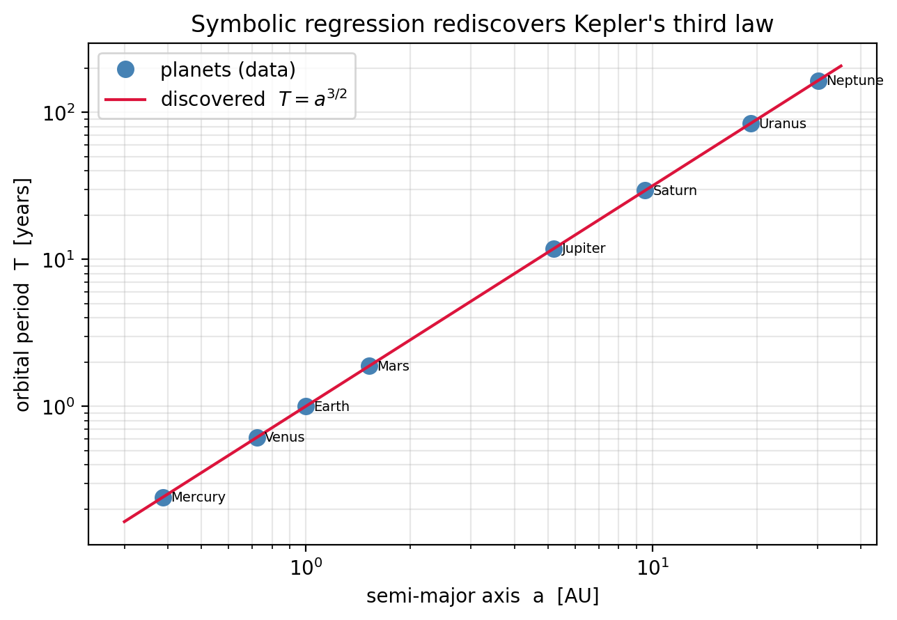
Feed the engine the semi-major axes and orbital periods of the eight planets — sixteen numbers, no units, no hints — and let it evolve. Read the result off the Pareto front:

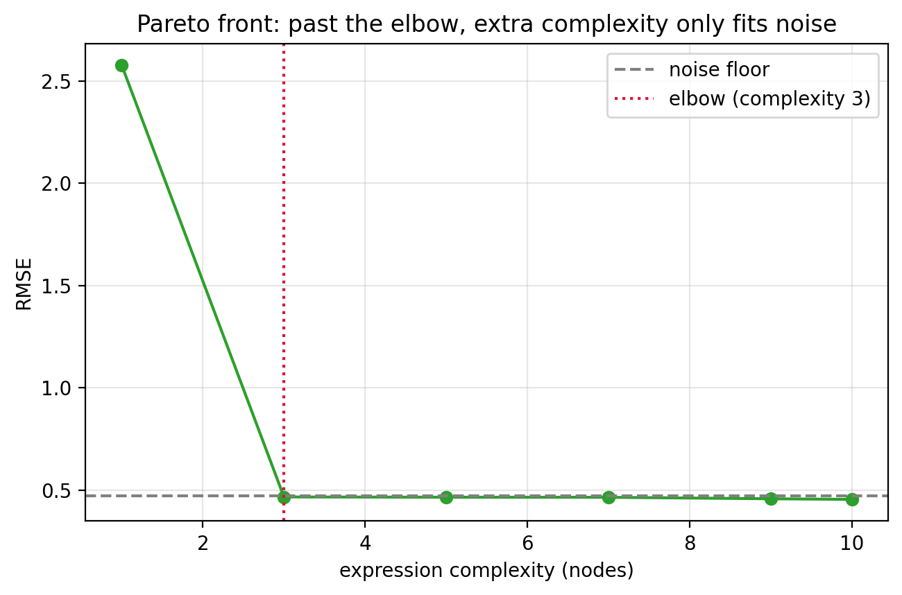
Rediscover T(a) from 8 planets   (operators: + - * / sqrt sq log)

  Pareto front  (accuracy vs complexity)
    complexity  1:   RMSE = 8.495 yr   R^2 = 0.9764    ~  5.385*a - 8.79
    complexity  2:   RMSE = 6.171 yr   R^2 = 0.9875    ~  0.183*a^2 + 4.80
    complexity  4:   RMSE = 0.008 yr   R^2 = 1.000000  ~  0.999*(a*sqrt(a))   <-- !
    complexity  7:   RMSE = 0.007 yr   R^2 = 1.000000  ~  ... + O(1e-3) noise terms
  chosen law (the elbow):   T = a*sqrt(a) = a^(3/2),   i.e.   T^2 = a^3
  log-log exponent fit:  1.4997      (Kepler's exponent = 3/2)

Noisy law   y = 2*x1*x2 + 0.5   (15% noise on 60 points)
    complexity  1:   RMSE = 2.577    ~  3.26*x2
    complexity  3:   RMSE = 0.467    ~  2.010*(x1*x2) + 0.537       <-- hits noise floor
    complexity  9:   RMSE = 0.458    ~  x2*(x1 + x1/log|x1+x2|)     <-- fitting noise
  noise floor RMSE = 0.472;   parsimony stops at complexity 3 = the true law

At complexity 1 the best it can do is a straight line, $R^2=0.976$ — decent, and completely wrong. At complexity 4 it finds $a\sqrt{a}=a^{3/2}$ and the error drops by three orders of magnitude to $R^2=1.000000$. Every more complicated expression on the front is that same law plus corrections at the $10^{-3}$ level — fitting the last digits of the tabulated radii, not physics. So the elbow is unmistakable, and it reads $T=a^{3/2}$, which is Kepler's third law, $T^2=a^3$. As a check, the raw log-log slope of the data is $1.4997$ against Kepler's exact $3/2$. The machine did in seconds what took Kepler the better part of a decade — not because it is smarter, but because it can try a million formulas without getting tired.

Why parsimony decides everything

Real data is noisy, and this is where a naive fit-the-error search destroys itself. Take $y=2x_1{x}_2+\frac{1}{2}$ and corrupt it with 15% noise. The Pareto front finds the true law — $2.010x_1{x}_2+0.537$ — at complexity 3, and that expression is the first to reach the noise floor (RMSE 0.467 against a floor of 0.472): there is nothing left to explain but the noise itself. Everything past the elbow proves the point by failing it — the search starts bolting on terms like $x_1/\log |x_1+x_2|$ that shave the RMSE by a percent while fitting pure randomness. The Pareto front is the guardrail: it makes the difference between a discovered law and an overfit one visible as a corner in a plot, rather than something you have to intuit.

What makes it hard, and what real engines add

• The search space is enormous. The number of trees grows super-exponentially in depth, and genetic programming is a stochastic walk through it — run it twice from different seeds and you may get different routes to the same law, or get stuck. Production tools (PySR) bolt simulated annealing and multi-population migration onto the evolution to search harder.
• The primitives must contain the answer. Kepler needs ​ in the operator set; drop it and no amount of evolution finds $a^{3/2}$ exactly. Choosing primitives is choosing the hypothesis class.
• Constants are the enemy of search. Discrete tree operations cannot tune a real number smoothly, which is why the linear-scaling trick above matters and why serious engines run a continuous optimizer on the constants inside every candidate.
• Physics has structure — use it. AI-Feynman leans on dimensional analysis, symmetry, and separability to shatter a hard formula into easy pieces, recovering dozens of textbook laws that raw genetic programming cannot touch. Units alone eliminate most of the search space before it starts.

The point, for a computational scientist

Kepler is a demonstration with a known answer; the reason to own this tool is the case where the answer is not known. Run a simulation — DFT adsorption energies across a catalyst series, excitation energies across a family of dyes, a transport coefficient across a phase diagram — and you have a table exactly like the planetary one, except no one has found the law yet. Symbolic regression is how you get an interpretable scaling relation out of your own output instead of a black-box fit: the superexchange $J\sim t^2/U$, a Sabatier volcano, a structure–property trend. Every DFT study that follows on this site is going to end by handing its numbers to this engine and asking what law they obey.

Reproduce it

scripts/gen_symbolic_regression.py is the whole engine — expression trees, tournament selection, subtree crossover and mutation, and the complexity-indexed Pareto front — in a few hundred lines with no dependencies beyond NumPy and SymPy (used only to pretty-print the winning tree). It rediscovers $T=a^{3/2}$ from the real planetary data ($R^2=1.000000$, exponent $1.4997$) and recovers $2x_1{x}_2+\frac{1}{2}$ from noisy samples without overfitting past the noise floor. Change the operator set or feed it your own table and watch the front move.