Lanczos learns the optimal basis: extracting the spectral measure

So theoretically this Lanczos process turns any symmetric matrix into a tridiagonal one, given a starting vector. This tridiagonal configuration corresponds to some kind of recurrence and there are a few canonical ones, the usual suspects, Legendre, Laguerre, Hermite, Chebyshev, etc. You don't always land on one of these nice cases though; a generic operator usually gives you a more exotic distribution. The idea is that you can take some starting matrix and from there you can recover the weighting function from the recurrence. You could have an operator that isn't quite one basis or the other, like a Hamiltonian where there is one operator diagonal in one basis and another diagonal in the other. Spectral methods are a good example of this.

An operator diagonal in neither basis

Here is the spectral-methods case with numbers. Discretize a 1D Hamiltonian $H=T+V$ on a periodic grid. The kinetic operator $T=-\frac{1}{2}{d}^2/d{x}^2$ is diagonal in the plane-wave (Fourier) basis — there it is just $\frac{1}{2}{k}^2$ — and dense in real space. The soft-Coulomb potential $V(x)=-1/\sqrt{x^2+a^2}$ is the mirror image: diagonal in real space, dense in the plane-wave basis. Measure the off-diagonal density of each (fraction of off-diagonal entries that are nonzero):

import numpy as np
N, L = 128, 15.0
x = np.linspace(-L, L, N, endpoint=False); dx = x[1] - x[0]
k = 2*np.pi*np.fft.fftfreq(N, d=dx); I = np.eye(N)

# Kinetic T = -1/2 d^2/dx^2 : diagonal in the plane-wave (Fourier) basis
Tk = np.diag(0.5*k**2)                                       # plane-wave basis
Tx = np.real(np.fft.ifft(0.5*k[:,None]**2 * np.fft.fft(I,0), 0))   # real-space

# Soft-Coulomb V(x) = -1/sqrt(x^2 + a^2) : diagonal in real space
a = 0.5
Vx = np.diag(-1/np.sqrt(x**2 + a**2))                        # real-space basis
W, Wi = np.fft.fft(I,0), np.fft.ifft(I,0)
Vk = W @ Vx @ Wi                                             # plane-wave basis

def offdensity(M, rel=1e-8):           # fraction of off-diagonal entries nonzero
    A = np.abs(M); m = A > rel*A.max(); np.fill_diagonal(m, False)
    return m.sum() / (M.size - N)

for name, M in [("T  real-space", Tx), ("T  plane-wave", Tk),
                ("V  real-space", Vx), ("V  plane-wave", Vk),
                ("H  real-space", Tx+Vx), ("H  plane-wave", Tk+Vk)]:
    print(f"{name:14s} off-diagonal density = {offdensity(M):.3f}")

T  real-space  off-diagonal density = 1.000
T  plane-wave  off-diagonal density = 0.000     <- kinetic is diagonal here
V  real-space  off-diagonal density = 0.000     <- potential is diagonal here
V  plane-wave  off-diagonal density = 1.000
H  real-space  off-diagonal density = 1.000     <- H = T + V is dense ...
H  plane-wave  off-diagonal density = 1.000     <- ... in both bases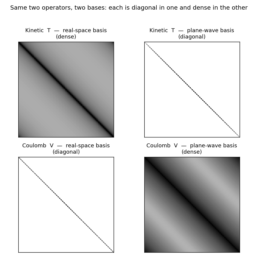

Each of $T$ and $V$ is diagonal in its own basis, but $H=T+V$ is dense in both — no off-the-shelf basis diagonalizes it. The basis that does is $H$'s own eigenbasis, which you do not have in advance. Lanczos builds a basis adapted to $H$ directly, from a starting vector, without committing to either analytic basis — and that adapted basis is the subject of the rest of this page.

1. Extracting the weight

Much like statistical sampling has some distributions, so do matrices. If you write a matrix using a certain rule it will have a certain distribution of eigenvalues. Eigenvalues are the roots of certain polynomials defined by a matrix. So what you really are doing is specifying a distribution of roots. In our case we have no knowledge of the generating process of the matrix, instead we are just trying to recover the distribution of the roots using the Lanczos process. It's like a decryption problem and you have some kind of algorithm to recover the information. In the terms of the field, this would be the weighting function or spectral measure. To be precise, it is weighted by your starting vector — each eigenvalue counts in proportion to $|⟨v_0|{\psi }_i⟩{|}^2$, how much $v_0$ overlaps it — so a localized $v_0$ gives a local version (in physics, the local density of states). In quantum mechanical or chemical contexts you will hear the word density of states, which is just a histogram of the eigenvalues of a system. All these fields have different names for the same thing. If you're in math you start talking about spectral measures, if you're in physics or chemistry it's all DOS. If you're in nuclear physics it's level density. Realistically you're just histogramming eigenvalues, which is not really the first thing you learn. And this Lanczos process is also performing an integral — the quadrature story below.

def lanczos(A, v0, m):                 # symmetric A, start v0, m steps
    n = len(v0); V = np.zeros((n, m)); a = np.zeros(m); b = np.zeros(m)
    V[:, 0] = v0 / np.linalg.norm(v0); bp = 0.0; vp = np.zeros(n)
    for j in range(m):
        w = A @ V[:, j]; a[j] = V[:, j] @ w; w = w - a[j]*V[:, j] - bp*vp
        for k in range(j): w -= (V[:, k] @ w) * V[:, k]   # reorthogonalize
        b[j] = np.linalg.norm(w)
        if b[j] < 1e-12 or j == m-1: break
        vp = V[:, j]; bp = b[j]; V[:, j+1] = w / b[j]
    return a, b, V

# The Jacobi matrix IS a compressed encoding of the spectral measure mu.
# Read it back: diagonalize T_m -> Ritz values (nodes) and squared first
# eigenvector components (weights). This discrete measure converges to mu.
def learned_weight(a, b, m):
    T = np.diag(a[:m]) + np.diag(b[:m-1], 1) + np.diag(b[:m-1], -1)
    theta, S = np.linalg.eigh(T)
    return theta, S[0, :]**2           # nodes, weights -> approximation of mu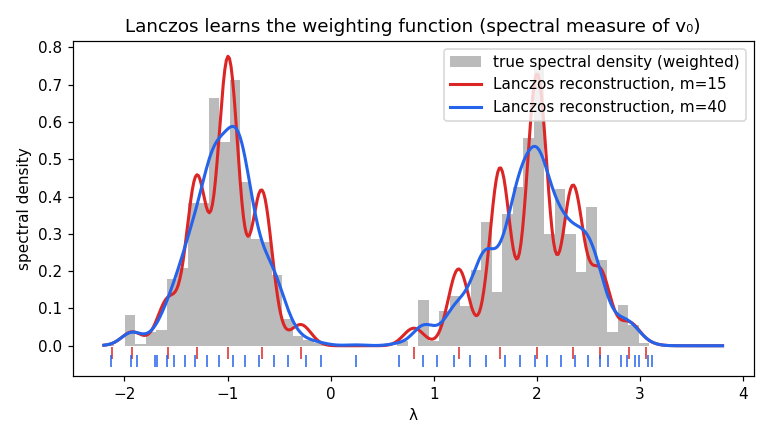

On an 800-dimensional operator with a deliberately bimodal spectrum, 40 Lanczos steps reconstruct the spectral density — both bumps, from 40 matrix-vector products. And it's exact in the moment sense: the reconstructed measure reproduces the first $2m$ moments of $\mu$ (checked: 16 moments matched to $3\times 10^{-10}$ at $m=8$). The Ritz nodes cluster where the spectral weight is and ignore the empty gap — the algorithm puts its resolution where the measure lives.

Lanczos is computing an integral

The integral promised at the end of p3 is concrete. The quantity $v_0^{\top }f(A)v_0$ — apply any function of $A$ to $v_0$ and project back — is an integral against the spectral measure:

So there is a curve being integrated, and it is worth seeing. The thing $f$ gets multiplied by is the density $\rho (\lambda )$: for a finite matrix it is a comb of spikes, one sitting on each eigenvalue with height equal to its $v_0$ weight; for a large system the spikes merge into the smooth density of states. Its running total is the cumulative $F(\lambda )$ — a staircase, or a smooth S-curve. Quadrature is sampling this curve: integrate $f$ against $\rho$ by evaluating at a few points.

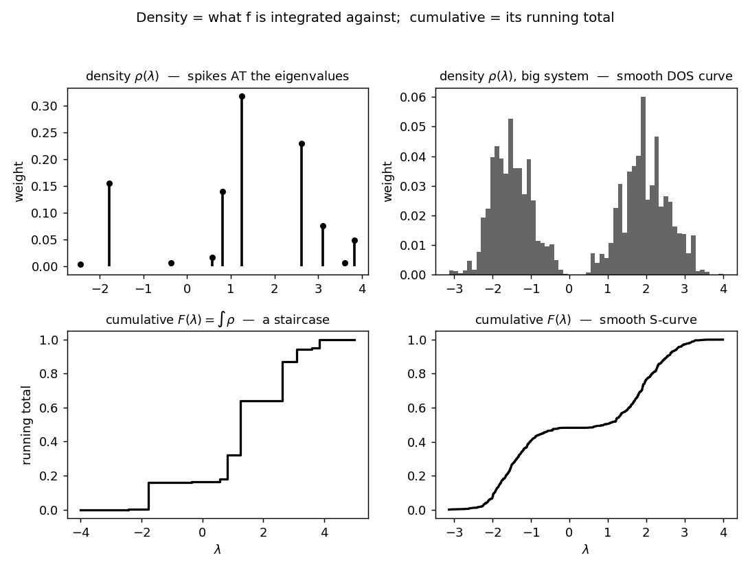
The sum runs over eigenvalues, weighted by the same $v_0$ overlaps from p3 — which is exactly what integrating $f$ against $\mu$ means. Lanczos evaluates this integral without diagonalizing $A$. Diagonalize the small tridiagonal $T_m$ instead: its eigenvalues ${\theta }_j$ are the nodes, the squared first components of its eigenvectors $w_j$ are the weights (Golub-Welsch). Then

is the $m$-point Gauss quadrature rule for $\mu$ — and an $m$-point Gauss rule is exact for polynomials up to degree $2m-1$. So $m$ Lanczos steps build the optimal $m$-point rule for integrating any function against a measure you never wrote down.

def gauss_rule(a, b, m):                 # decode T_m into a quadrature rule
    T = np.diag(a[:m]) + np.diag(b[:m-1], 1) + np.diag(b[:m-1], -1)
    theta, S = np.linalg.eigh(T)
    return theta, S[0, :]**2             # nodes (Ritz values), weights (Golub-Welsch)

def integrate(f, A, v0, m):              # m-point Gauss estimate of  int f dmu
    a, b = lanczos(A, v0, m)
    theta, w = gauss_rule(a, b, m)
    return np.sum(w * f(theta))

# the exact value is just the bilinear form  v0^T f(A) v0  =  int f dmu
ev, Q = np.linalg.eigh(A)
exact = lambda f: v0 @ (Q @ (f(ev) * (Q.T @ v0)))

for m in [1, 2, 4, 6, 8]:
    approx = integrate(lambda x: np.exp(-0.4*x), A, v0, m)
    print(m, approx, abs(approx - exact(lambda x: np.exp(-0.4*x))))

# f(x) = x**5   (a degree-5 polynomial: Gauss is exact once 5 <= 2m-1, i.e. m >= 3)
m=2   Gauss = 142.566807   exact = 165.448077   err = 2.3e+01
m=3   Gauss = 165.448077   exact = 165.448077   err = 8.5e-14   <- exact at m=3
m=4   Gauss = 165.448077   exact = 165.448077   err = 1.4e-13

# f(x) = exp(-0.4 x)   (smooth, not a polynomial)
m=1   err = 4.4e-01
m=2   err = 7.8e-03
m=4   err = 7.2e-07
m=6   err = 8.7e-12
m=8   err = 2.2e-16   <- machine precision in 8 matrix-vector products

Both regimes show up in the run. A degree-5 polynomial is integrated exactly the instant $m=3$, because $5\le 2\cdot 3-1$ — three Lanczos steps, machine-precision integral. A smooth non-polynomial has no exact degree, so it converges instead, hitting machine precision in eight steps. Either way the histogram of p3 and the integral against that histogram are the same Jacobi matrix read two ways: bin it and you get the density of states; integrate against it and you get a Gauss rule.

2. The adapted basis is optimal

"Optimal" is not hand-waving here; it's a one-line identity. For any function $g$, $\Vert g(A)v_0{\Vert }^2=v_0^{\top }g(A{)}^2{v}_0=\int |g(x){|}^{2}d\mu (x)$. So approximating $f(A)v_0$ by a degree-$m$ polynomial $p_m(A)v_0$ has error

which is the $L^2(\mu )$ approximation error. The $L^2(\mu )$-optimal degree-$m$ polynomial is the truncated expansion in $\mu$'s orthogonal polynomials — exactly what Lanczos produces. So the adapted basis is the optimal one for representing any function of $A$ applied to $v_0$, and it wins precisely because it spends its resolution only where $\mu$ has weight. A fixed basis (Chebyshev on an interval around the spectrum) wastes degrees of freedom on the empty gap.

# ADAPTED basis: f(A)v0 ~= ||v0|| * V_m @ f(T_m) @ e1, applying f to the
# small m x m tridiagonal via its eigendecomposition (cheap; m is tiny).
def lanczos_apply(f, A, v0, m):
    a, b, V = lanczos(A, v0, m)                  # lanczos() from above
    T = np.diag(a[:m]) + np.diag(b[:m-1], 1) + np.diag(b[:m-1], -1)
    th, S = np.linalg.eigh(T)                    # eigendecompose T_m
    fT = S @ np.diag(f(th)) @ S.T                # f(T_m)
    e1 = np.zeros(m); e1[0] = 1.0
    return np.linalg.norm(v0) * V[:, :m] @ (fT @ e1)

# FIXED basis: truncated Chebyshev series of f, applied to A by the Chebyshev
# three-term recurrence on vectors (no eigendecomposition of A at all).
def cheb_apply(ck, A, v0, m, lo, hi):
    c, d = (hi + lo) / 2, (hi - lo) / 2
    At = (A - c * np.eye(len(v0))) / d           # map spectrum into [-1, 1]
    Tkm1 = v0.copy(); Tk = At @ v0
    y = ck[0] * Tkm1 + ck[1] * Tk
    for k in range(2, m + 1):
        Tkp1 = 2 * (At @ Tk) - Tkm1              # Chebyshev recurrence
        y += ck[k] * Tkp1; Tkm1, Tk = Tk, Tkp1
    return y

# Key identity:  ||g(A) v0||^2 = integral |g(x)|^2 d mu(x).  So minimizing the
# Euclidean error of p(A)v0 IS minimizing the L2(mu) error of p approximating
# f -- and the L2(mu)-optimal degree-m polynomial is the truncation in mu's
# orthogonal polynomials, which is exactly what lanczos_apply builds.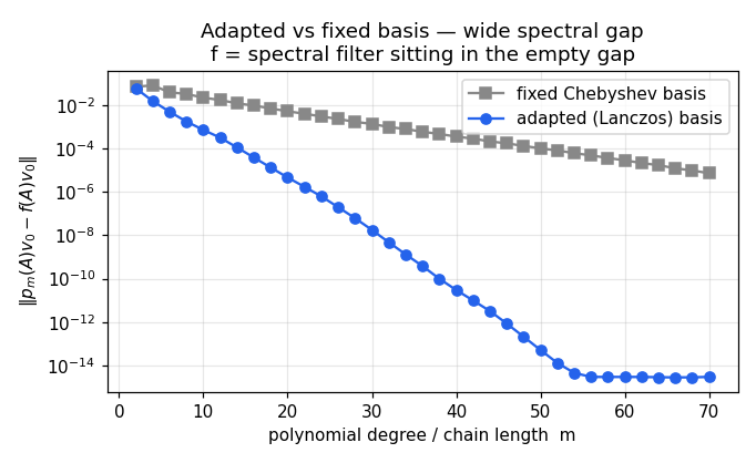

The test: approximate $f(A)v_0$ where $f$ is a spectral filter (a Fermi step that selects the lower cluster), with the step sitting in a wide empty gap between clusters at $\lambda =-2$ and $\lambda =3$. The fixed Chebyshev basis must resolve that sharp step even though no spectral weight is there; the adapted basis doesn't care about the gap at all, only about the two clusters where $f\approx 1$ and $f\approx 0$ are nearly constant. The result is lopsided: the adapted basis descends geometrically to $3\times 10^{-11}$ by degree $m=40$ and hits machine precision ($\sim 3\times 10^{-15}$) by $m\approx 56$, while Chebyshev is still at $4\times 10^{-4}$ at $m=40$ — about seven orders of magnitude better, with the gap widening at every degree. The wider the empty gap, the more resolution Chebyshev wastes on it and the bigger the adapted basis's edge.

One thing to read correctly on the plot: the adapted curve flattens at the bottom around $10^{-15}$. That's the roundoff floor, not a feature of the method — once the error reaches machine precision it can only jitter at the level of double-precision noise, which a log axis magnifies into apparent oscillation. The descent itself is clean and monotone; the flat tail is just the floor.

3. The v₀ knob: you choose what the weight emphasizes

The measure isn't fixed by $A$ alone — it depends on $v_0$. Different starting vectors put weight on different parts of the spectrum, so you can steer the learned weight toward the region you care about. Start from a vector pre-filtered toward the lower cluster and the learned weight concentrates there; start from one aimed high and it moves.

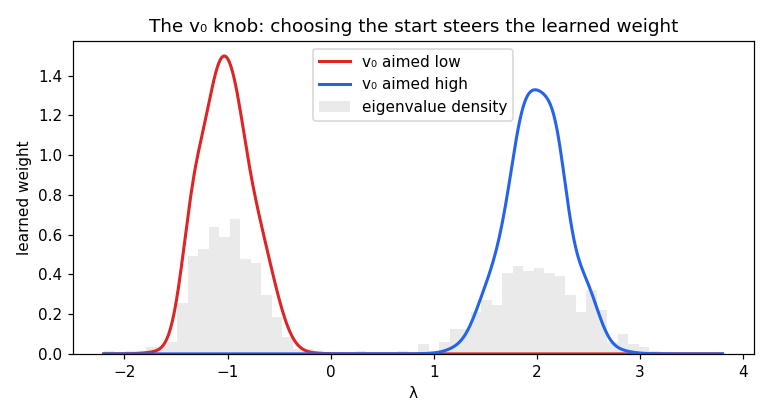
This is the design freedom in "learn the optimal weight": pick $v_0$ (or a block of starting vectors, giving a matrix-valued measure and a richer adapted basis) to focus the polynomials where your problem demands accuracy — a spectral window, a target observable, the occupied states of a Hamiltonian. The same operator yields different optimal bases for different questions.

4. Non-symmetric operators: biorthogonal Lanczos and formal polynomials

For a non-symmetric $A$ there is no single orthonormal basis that tridiagonalizes it. Two-sided (biorthogonal) Lanczos builds two sequences — right vectors $v_j$ and left vectors $w_j$ — that are biorthogonal, $w_i^{\top }{v}_j={\delta }_{ij}$, and make $W^{\top }AV=T$ tridiagonal. The recurrence coefficients are now formal orthogonal polynomials with respect to a bilinear moment functional — generally a signed or complex measure, not a positive one. Favard's theorem fails: there's no guarantee of an underlying positive measure, and the coefficients ${\delta }_j={\beta }_j{\gamma }_j$ come out signed.

def two_sided(A, v1, w1, m):           # NON-symmetric A; require w1^T v1 = 1
    # builds biorthogonal V (right), W (left): W^T V = I, W^T A V = T tridiagonal
    ...
    delta = wh @ vh                    # the next coefficient: SIGNED or complex
    # full biorthogonalization each step -- without it the bases blow up:
    for _ in range(2):
        vh -= V[:, :j+1] @ (W[:, :j+1].T @ vh)
        wh -= W[:, :j+1] @ (V[:, :j+1].T @ wh)
    ...

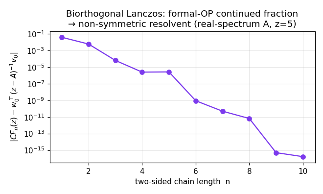
On a real-spectrum non-symmetric matrix, the two-sided continued fraction converges to the bilinear resolvent $w_0^{\top }(z1-A{)}^{-1}{v}_0$ — from $4\times 10^{-2}$ at one level to $2\times 10^{-16}$ at full dimension. Two features show up that the symmetric case doesn't have. The convergence is not monotone (a small bump near $n=4$) — formal-orthogonal-polynomial Padé approximants have no monotonicity guarantee. And the coefficients are signed (${\delta }_j=-4.12,-5.48,-0.18,\dots$), the signature of a non-positive measure. The method is also unstable without explicit re-biorthogonalization (the bases lose biorthogonality and blow up); a bare two-sided Lanczos on a wildly non-normal matrix diverges, and serious breakdowns (${\delta }_j=0$ with nonzero vectors) need look-ahead Lanczos to step over. This is exactly the machinery behind non-symmetric model-order reduction (PVL, PRIMA).

What this is

Pull the four pieces together. Lanczos, fed an operator and a vector, learns the spectral measure (part 1), and the orthogonal polynomials of that measure are the optimal basis for any function of the operator (part 2). The starting vector is a knob that aims the measure (part 3). The biorthogonal version extends it to non-symmetric operators at the cost of positivity and stability (part 4). The named families and quadratures are the classical-weight special cases; on a real operator you get a bespoke basis tuned to its spectrum. The continued fraction is the resolvent, the Gauss rule is the spectral-density estimate, the Padé is the moment match — all of it the orthogonal polynomials of the measure Lanczos learned.

As a falsifiable claim: the orthogonal polynomials of $v_0$'s spectral measure are the $L^2(\mu )$-optimal polynomial basis for approximating $f(A)v_0$, and Lanczos produces them. The experiment is part 2 — the adapted basis beats any fixed basis in the spectral-measure norm, widening with degree. It would be falsified by a fixed basis that matched or beat the adapted one in $L^2(\mu )$ at every degree, which the optimality identity forbids.

Related on this site

• Lanczos ↔ continued fractions — the classical-orthogonal-polynomial capstone this page inverts.
• Lanczos iteration — the base algorithm.
• Bi-orthogonal Lanczos — the two-sided variant for non-symmetric operators.
• Padé via Lanczos — the adapted basis put to work in model-order reduction.