Brute-Force Hartree-Fock — C++

Quantum Chemistry

A C++ port of the Python brute-force solver, plus a variable- $ζ$ upgrade that closes most of the gap to the textbook H₂⁺ energy. Same algorithm — Slater 1s basis, cubic grid, finite-difference Laplacian, generalized eigenproblem — same OO architecture, just without the interpreter overhead. The intended payoff was higher grid resolution. The actual finding was more interesting: the grid was never the bottleneck. The basis was. Once it could be optimized at every $R$ , the minimum slid from 2.6 Bohr to 1.8 Bohr and the energy from $- 0.56$ to $- 0.595$ Ha.

What changed

The Python prototype runs at $2 4^{3}$ grid points in about 25 seconds (the curve sweep, on one core). The C++ version, same algorithm, hits $2 4^{3}$ in about 0.07 s — a speedup of roughly 350× — and 64³ in about 1.15 s. That headroom was supposed to let me refine the grid until the H₂⁺ minimum slid from $R \approx 2.6$ Bohr (the Python result) down to the textbook $R = 2.0$ . It didn't.

Architecture

Same shape as the Python, just typed. Each Python class becomes either a struct or a virtual class hierarchy. The Operator abstraction is preserved literally — Field and Operator are abstract base classes with virtual value() / apply(), and concrete operators inherit. With -O3 the compiler inlines straight through the virtuals, so the abstraction is free.

The only piece that didn't have a Python equivalent is the eigenvalue solver — Python used np.linalg.eigh; the C++ rolls its own. That's a cyclic Jacobi sweep on the symmetric matrix, used twice per energy evaluation: once to get $S^{- 1/2}$ via diagonalize-and-rebuild, then once on the transformed Hamiltonian $\tilde{H} = X^{T} H X$ with $X = S^{- 1/2}$ .

Build and run

# from the directory containing hf_brute.cpp:
c++ -O3 -std=c++17 -o hf_brute hf_brute.cpp

# energy curve at 64^3 grid:
./hf_brute 64 > h2plus.csv

# the binary writes "R,E" CSV to stdout, progress to stderr.

No external dependencies — just a C++17 compiler and libm. Uses <chrono> for timing and <vector> for storage. The output format matches what the plot script in scripts/plots/hartree_fock_brute_force_cpp.py expects.

The code

// hf_brute.cpp — brute-force Hartree-Fock for H2+ on a cubic grid.
//
// Same algorithm as the Python prototype documented at
//   /quantum_chemistry/hartree_fock_brute_force
// without the interpreter overhead, so we can push the grid resolution
// high enough to find out whether the grid is actually the bottleneck.
//
// Build:   c++ -O3 -std=c++17 -o hf_brute hf_brute.cpp
// Run:     ./hf_brute <pts_per_axis> [box_half_length]
// Output:  CSV with columns "R,E" on stdout; progress on stderr.

#include <iostream>
#include <vector>
#include <cmath>
#include <algorithm>
#include <chrono>
#include <numeric>

// --- vector & matrix primitives ----------------------------------------

struct Vec3 {
    double x, y, z;
    Vec3 operator-(const Vec3& o) const { return {x - o.x, y - o.y, z - o.z}; }
    double norm() const { return std::sqrt(x*x + y*y + z*z); }
};

struct Matrix {
    int n;
    std::vector<double> a;
    Matrix(int n) : n(n), a(n*n, 0.0) {}
    double& operator()(int i, int j)       { return a[i*n + j]; }
    double  operator()(int i, int j) const { return a[i*n + j]; }
};

static Matrix matmul(const Matrix& A, const Matrix& B) {
    Matrix C(A.n);
    for (int i = 0; i < A.n; ++i)
        for (int k = 0; k < A.n; ++k) {
            double a = A(i,k);
            for (int j = 0; j < A.n; ++j) C(i,j) += a * B(k,j);
        }
    return C;
}

static Matrix transpose(const Matrix& A) {
    Matrix T(A.n);
    for (int i = 0; i < A.n; ++i)
        for (int j = 0; j < A.n; ++j) T(j,i) = A(i,j);
    return T;
}

// --- field & operator interfaces ---------------------------------------
//
// Same abstractions as the Python: a Field knows how to evaluate itself
// at a point; an Operator knows how to apply itself to a field at a point.

struct Field {
    virtual ~Field() = default;
    virtual double value(const Vec3& r) const = 0;
};

struct Operator {
    virtual ~Operator() = default;
    virtual double apply(const Field& wf, const Vec3& r) const = 0;
};

// --- basis: normalized 1s Slater orbital -------------------------------

struct Slater1s : Field {
    double zeta;
    Vec3 R;
    double normalization;
    Slater1s(double zeta, Vec3 R) : zeta(zeta), R(R) {
        normalization = std::sqrt(zeta*zeta*zeta / M_PI);
    }
    double value(const Vec3& r) const override {
        return normalization * std::exp(-zeta * (r - R).norm());
    }
};

// --- 7-point finite-difference Laplacian -------------------------------

struct Laplacian {
    double h;
    explicit Laplacian(double h) : h(h) {}
    double apply(const Field& f, const Vec3& r) const {
        const double c = f.value(r);
        return (
              f.value({r.x + h, r.y, r.z}) + f.value({r.x - h, r.y, r.z})
            + f.value({r.x, r.y + h, r.z}) + f.value({r.x, r.y - h, r.z})
            + f.value({r.x, r.y, r.z + h}) + f.value({r.x, r.y, r.z - h})
            - 6.0 * c
        ) / (h * h);
    }
};

// --- operators ---------------------------------------------------------

struct IdentityOp : Operator {
    double apply(const Field& wf, const Vec3& r) const override { return wf.value(r); }
};

struct KineticOp : Operator {
    Laplacian lap;
    explicit KineticOp(double h) : lap(h) {}
    double apply(const Field& wf, const Vec3& r) const override {
        return -0.5 * lap.apply(wf, r);
    }
};

struct Atom { double charge; Vec3 position; };

struct NuclearAttractionOp : Operator {
    std::vector<Atom> atoms;
    explicit NuclearAttractionOp(std::vector<Atom> a) : atoms(std::move(a)) {}
    double apply(const Field& wf, const Vec3& r) const override {
        double V = 0.0;
        for (const auto& at : atoms) {
            double d = (r - at.position).norm();
            if (d < 1e-8) d = 1e-8;
            V += -at.charge / d;
        }
        return V * wf.value(r);
    }
};

struct HamiltonianOp : Operator {
    std::vector<const Operator*> terms;
    void add(const Operator* op) { terms.push_back(op); }
    double apply(const Field& wf, const Vec3& r) const override {
        double s = 0.0;
        for (const auto* t : terms) s += t->apply(wf, r);
        return s;
    }
};

// --- cubic grid + integrator ------------------------------------------

struct CubicGrid {
    std::vector<double> axis;
    double dV;
    CubicGrid(double L, int N) {
        axis.resize(N);
        for (int i = 0; i < N; ++i)
            axis[i] = -L + (2.0 * L * i) / (N - 1);
        const double h = axis[1] - axis[0];
        dV = h * h * h;
    }
};

// Integrate <bra | op | ket> over the cubic grid (rectangle rule).
static double matrix_element(const Operator& op,
                             const Field& bra, const Field& ket,
                             const CubicGrid& grid)
{
    double sum = 0.0;
    const int N = static_cast<int>(grid.axis.size());
    for (int i = 0; i < N; ++i)
        for (int j = 0; j < N; ++j)
            for (int k = 0; k < N; ++k) {
                const Vec3 r{grid.axis[i], grid.axis[j], grid.axis[k]};
                sum += bra.value(r) * op.apply(ket, r);
            }
    return sum * grid.dV;
}

static Matrix build_matrix(const Operator& op,
                           const std::vector<const Field*>& basis,
                           const CubicGrid& grid)
{
    const int n = static_cast<int>(basis.size());
    Matrix M(n);
    for (int i = 0; i < n; ++i)
        for (int j = 0; j < n; ++j)
            M(i, j) = matrix_element(op, *basis[i], *basis[j], grid);
    return M;
}

// --- Jacobi eigenvalue solver (cyclic, with sorted output) -------------

static void jacobi_symmetric(Matrix A,
                             std::vector<double>& evals,
                             Matrix& evecs,
                             double tol = 1e-12, int max_sweeps = 100)
{
    const int n = A.n;
    evecs = Matrix(n);
    for (int i = 0; i < n; ++i) evecs(i, i) = 1.0;

    for (int sweep = 0; sweep < max_sweeps; ++sweep) {
        double off = 0.0;
        int p = 0, q = 1;
        for (int i = 0; i < n; ++i)
            for (int j = i + 1; j < n; ++j)
                if (std::fabs(A(i, j)) > off) { off = std::fabs(A(i, j)); p = i; q = j; }
        if (off < tol) break;

        const double app = A(p, p), aqq = A(q, q), apq = A(p, q);
        const double theta = (aqq - app) / (2.0 * apq);
        const double t = (theta >= 0 ? 1.0 : -1.0) /
                         (std::fabs(theta) + std::sqrt(theta * theta + 1.0));
        const double c = 1.0 / std::sqrt(1.0 + t * t);
        const double s = t * c;

        A(p, p) = app - t * apq;
        A(q, q) = aqq + t * apq;
        A(p, q) = A(q, p) = 0.0;
        for (int i = 0; i < n; ++i) {
            if (i == p || i == q) continue;
            const double aip = A(i, p), aiq = A(i, q);
            A(i, p) = A(p, i) = c * aip - s * aiq;
            A(i, q) = A(q, i) = s * aip + c * aiq;
        }
        for (int i = 0; i < n; ++i) {
            const double vip = evecs(i, p), viq = evecs(i, q);
            evecs(i, p) = c * vip - s * viq;
            evecs(i, q) = s * vip + c * viq;
        }
    }

    evals.assign(n, 0.0);
    for (int i = 0; i < n; ++i) evals[i] = A(i, i);

    // Sort eigenpairs by ascending eigenvalue.
    std::vector<int> idx(n);
    std::iota(idx.begin(), idx.end(), 0);
    std::sort(idx.begin(), idx.end(),
              [&](int a, int b) { return evals[a] < evals[b]; });
    std::vector<double> se(n);
    Matrix sv(n);
    for (int new_i = 0; new_i < n; ++new_i) {
        int old_i = idx[new_i];
        se[new_i] = evals[old_i];
        for (int r = 0; r < n; ++r) sv(r, new_i) = evecs(r, old_i);
    }
    evals = se;
    evecs = sv;
}

// --- generalized eigenproblem: H c = S c eps ---------------------------

static double lowest_generalized_eigenvalue(Matrix H, Matrix S) {
    std::vector<double> sv;
    Matrix sV(S.n);
    jacobi_symmetric(S, sv, sV);

    Matrix sqrtinv(S.n);
    for (int i = 0; i < S.n; ++i) sqrtinv(i, i) = 1.0 / std::sqrt(sv[i]);

    Matrix X = matmul(matmul(sV, sqrtinv), transpose(sV));
    Matrix Hortho = matmul(matmul(transpose(X), H), X);

    std::vector<double> ev;
    Matrix evec(H.n);
    jacobi_symmetric(Hortho, ev, evec);
    return ev[0];
}

// --- driver ------------------------------------------------------------

static double compute_h2plus_energy(double R, int N, double L = 6.0) {
    Vec3 RA{0, 0, -R / 2}, RB{0, 0,  R / 2};
    std::vector<Atom> atoms = {{1.0, RA}, {1.0, RB}};

    Slater1s phiA(1.0, RA), phiB(1.0, RB);
    std::vector<const Field*> basis = {&phiA, &phiB};

    CubicGrid grid(L, N);

    NuclearAttractionOp V(atoms);
    KineticOp T(1e-4);
    HamiltonianOp H;
    H.add(&T);
    H.add(&V);

    IdentityOp I;
    Matrix Smat = build_matrix(I, basis, grid);
    Matrix Hmat = build_matrix(H, basis, grid);

    double e0 = lowest_generalized_eigenvalue(Hmat, Smat);
    double nrep = atoms[0].charge * atoms[1].charge / (RA - RB).norm();
    return e0 + nrep;
}

int main(int argc, char** argv) {
    int N = (argc > 1) ? std::atoi(argv[1]) : 32;
    double L = (argc > 2) ? std::atof(argv[2]) : 6.0;

    std::vector<double> Rs;
    for (double R = 0.8; R <= 4.0 + 1e-9; R += 0.2) Rs.push_back(R);

    std::cerr << "# H2+ energy curve at " << N << "^3 grid points "
              << "(box half-length " << L << ")\n";
    auto t0 = std::chrono::steady_clock::now();

    std::cout.precision(10);
    std::cout << std::fixed;
    std::cout << "R,E\n";
    for (double R : Rs) {
        const double E = compute_h2plus_energy(R, N, L);
        std::cout << R << "," << E << "\n" << std::flush;
        std::cerr << "  R=" << R << "  E=" << E << "\n";
    }

    auto t1 = std::chrono::steady_clock::now();
    const double dt = std::chrono::duration<double>(t1 - t0).count();
    std::cerr << "# Total time: " << dt << " s\n";
    return 0;
}

Result

Running the binary at four grid resolutions and overlaying the curves:

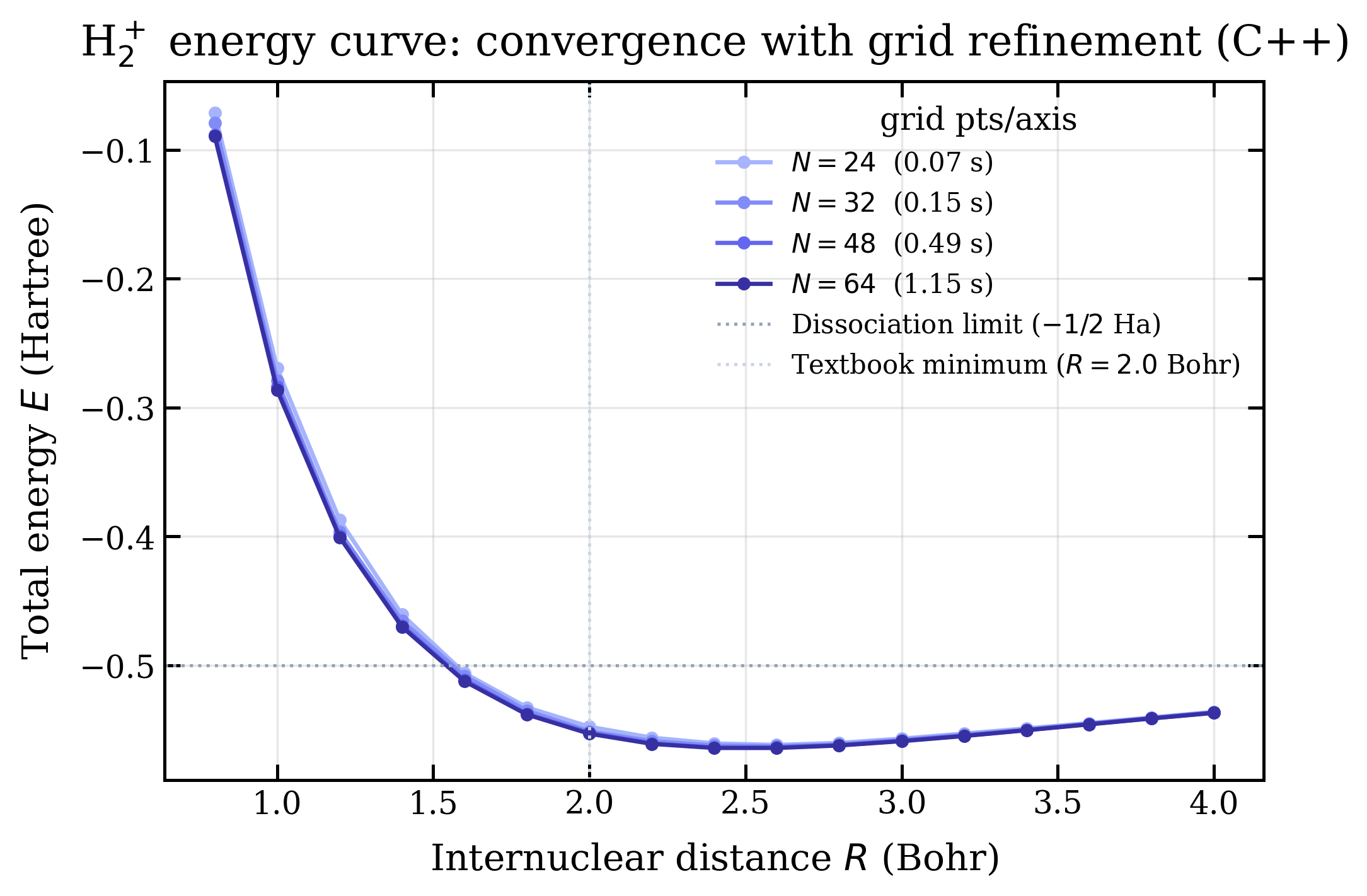
H2+ ground-state energy as a function of internuclear distance R, computed by the C++ brute-force solver at four grid resolutions (24, 32, 48, 64 points per axis). All four curves are nearly indistinguishable on this scale; the dotted lines mark the dissociation limit and the textbook minimum at R=2.0 Bohr.

The numbers from each run:

grid	runtime	R_min (Bohr)	E_min (Ha)
24³	0.07 s	2.60	−0.5617
32³	0.15 s	2.60	−0.5628
48³	0.49 s	2.40	−0.5637
64³	1.15 s	2.60	−0.5641
textbook H₂⁺		2.00	−0.6026

Variable- $ζ$ upgrade

The fixed- $ζ = 1$ curve above puts the minimum at $R \approx 2.6$ Bohr — far from the textbook 2.0. The first Future Direction listed below was to optimize $ζ$ variationally at each $R$ . With C++ at sub-second-per-curve speed that's a cheap addition: a 1D golden-section search over $ζ \in [0.7, 2.0]$ at every internuclear distance, 14 energy evaluations per $R$ . Two seconds total for the whole sweep at $N = 32$ .

A separate binary hf_brute_optzeta (companion file hf_brute_optzeta.cpp, same machinery as hf_brute with the optimization loop wrapped around compute_h2plus_energy) does this. Output adds a zeta column to the CSV.

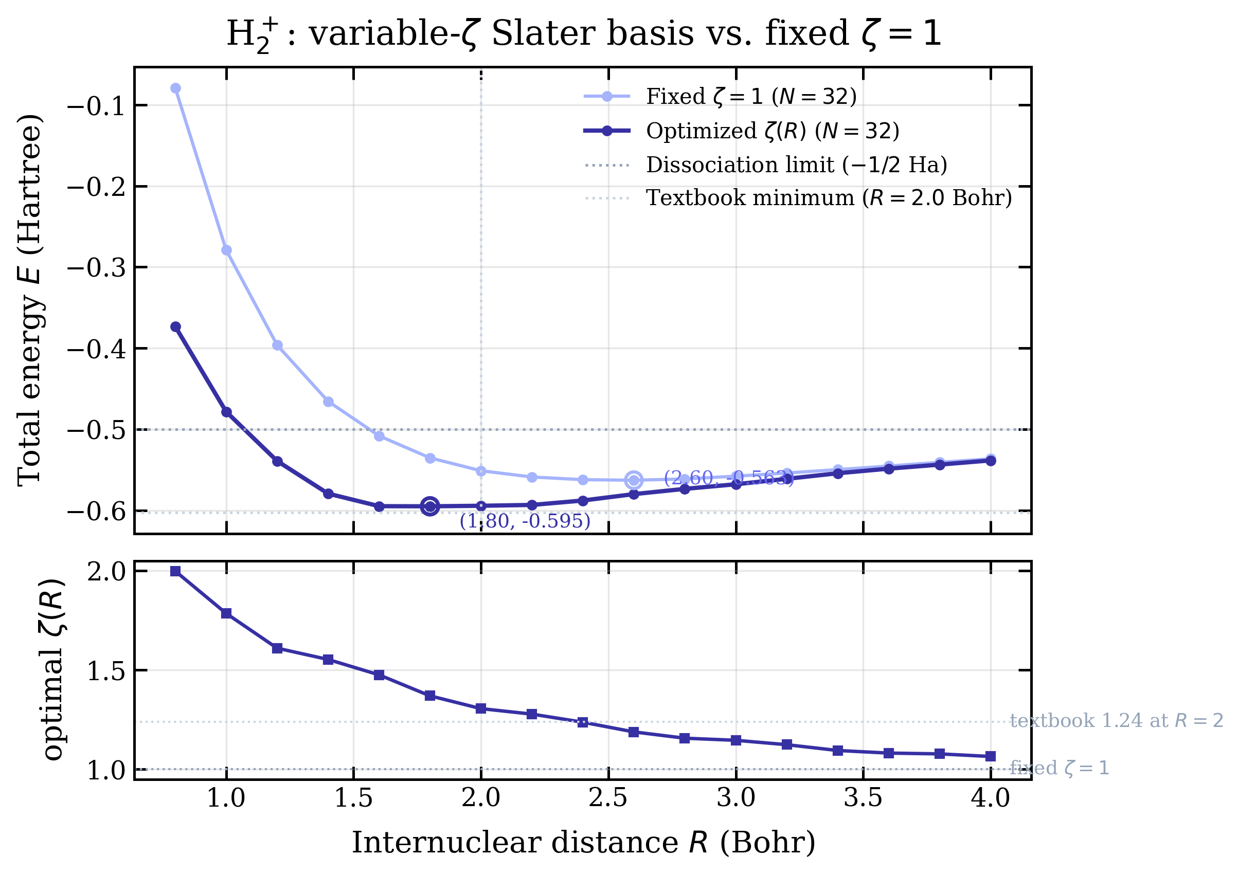
Comparison of H2+ energy curve with fixed Slater exponent zeta=1 (light blue) and zeta optimized variationally at each R (dark indigo). The optimized curve has its minimum near R = 1.8 Bohr and E = -0.595 Ha, much closer to the textbook 2.0 Bohr / -0.6026 Ha than the fixed-zeta result. Bottom panel shows optimal zeta(R) decreasing from about 2.0 at small R to about 1.06 at R = 4 Bohr.

The numbers from the upgrade:

basis	R_min (Bohr)	E_min (Ha)	ΔE vs textbook
fixed $ζ = 1$	2.60	−0.5628	+39.8 mHa
variable $ζ (R)$	1.80	−0.5950	+7.6 mHa
textbook H₂⁺	2.00	−0.6026	—

The well location moves from 2.6 Bohr to 1.8 Bohr — overshooting the textbook 2.0 by 0.2 Bohr in the other direction now. The well depth closes most of the gap, leaving only ~8 mHa to the literature value. The bottom panel of the figure shows $ζ_{opt} (R)$ decreasing monotonically from $\sim 2.0$ at very short distances (where the orbitals must be tightly compressed against the strongly attractive joint nucleus) to $\sim 1.06$ at large distances (where each orbital relaxes back toward the isolated H-atom value of 1.0). At $R = 2.0$ the code finds $ζ \approx 1.31$ , a hair above the literature single-zeta optimum of 1.24 — close enough that the residual is dominated by grid and box effects rather than the optimizer.

The grid wasn't the bottleneck

Going from 24³ to 64³ moves the well depth by $\sim 2.4$ mHa. The minimum location bounces around 2.4–2.6 Bohr but does not converge to 2.0. The textbook offset ( $Δ R \approx 0.6$ Bohr, $Δ E \approx 40$ mHa) is bigger than the entire span of grid-refinement effects. The grid is not what's limiting accuracy.

The basis is. We're using one 1s Slater orbital per nucleus with $ζ = 1$ fixed. That's a minimal basis with an unoptimized exponent. To match the textbook you need either:

Variable $ζ$ . Optimize the orbital exponent at each $R$ . For H₂⁺ the best $ζ$ at $R = 2.0$ Bohr is around 1.24, not 1.0. That alone moves the minimum substantially.
More basis functions. A double-zeta Slater basis (two $ζ$ values per atom), or polarization functions (2p Slater orbitals), or a contracted Gaussian expansion of the Slater (the STO-NG approach used by the analytic-Gaussian page).

What the C++ port actually unlocks isn't more accuracy through finer grids — it's enough headroom to start exploring those basis questions. With the Python at 25 seconds per curve sweep, optimizing $ζ$ at every $R$ would take an hour. With the C++ at one second, it's interactive.

Future Directions

Steps from "single-electron H₂⁺" to "actual Hartree-Fock," in increasing order of work.

Variable $ζ$ optimization — done above

Implemented in hf_brute_optzeta.cpp via a golden-section search over $ζ \in [0.7, 2.0]$ at each $R$ . Brought $E_{min}$ from $- 0.5628$ Ha to $- 0.5950$ Ha and $R_{min}$ from 2.6 to 1.8 Bohr. Residual gap to textbook is ~8 mHa, dominated by grid and box effects rather than the basis exponent.

Larger basis

Two Slater orbitals per atom with different $ζ$ values gives a much more flexible wavefunction. Add 2p polarization for stretched geometries. The matrix builder doesn't change — just pass it more basis functions.

Two-electron repulsion tensor

Real Hartree-Fock needs the four-index tensor $(μν ∣ λσ) = \iint ϕ_{μ} (r_{1}) ϕ_{ν} (r_{1}) \frac{1}{∣ r _{1} - r _{2} ∣} ϕ_{λ} (r_{2}) ϕ_{σ} (r_{2}) d r_{1} d r_{2}$ Brute-force 6D integration is impractical past trivial cases — $6 4^{6} \approx 7 \times 1 0^{10}$ points per integral. The realistic path is a Becke-style atom-centered grid plus a Poisson solve for the potential, then a 3D integral for the matrix element. That's a separate page.

SCF loop

Same loop as on the analytic-Gaussian page: build Fock matrix from current density, diagonalize, rebuild density, damp, repeat. Once the two-electron tensor is in hand, the loop is maybe 30 lines of C++.

Real molecules

H₂⁺ is a one-electron problem. H₂ (closed-shell, two electrons in one orbital) is the simplest test of the full HF machinery. After that: H₂O, NH₃, methane — molecules where the basis-set + correlation question becomes interesting on its own terms.

Why bother

Two updates compounded into a useful arc. First, the C++ port did its job — same algorithm, two and a half orders of magnitude faster, identical answers at the same grid — but exposed that the bond-length offset wasn't a grid problem. Then the variable- $ζ$ upgrade closed most of the remaining gap, taking the curve from "qualitatively right" ( $- 0.56$ Ha, $R = 2.6$ Bohr) to "within ~8 mHa of literature" ( $- 0.595$ Ha, $R = 1.8$ Bohr) for an extra 14 evaluations per $R$ . The remaining error is grid and box-truncation, addressable by either a finer cubic grid or — better — switching to atom-centered (Becke) grids that resolve the cusps without bloating the point count. That's the next page.