“Know how to solve every problem that has been solved.” “What I cannot create, I do not understand.” — Richard Feynman

Lanczos ↔ continued fractions (cycling reader)

Cycling

A document in the cycling-rephrasings format: each paragraph below has multiple framings of the same claim. The default view shows one framing per paragraph; click any paragraph to cycle to another framing of its claim. The outline view (top button) hides all bodies and shows the argument's skeleton — the overview sequence — for fast skimming. Each card has a copy button (top-right) that grabs the framing you're currently looking at.

Click a paragraph to cycle through its alternative framings.

There are three facts at work. First, the inverse of a tridiagonal matrix has a closed-form expression that happens to look like a continued fraction. Second, Lanczos — given any symmetric operator and a starting vector — builds an orthonormal basis in which that operator IS tridiagonal. Third, matrix elements of the resolvent in that basis project onto matrix elements of the tridiagonal's inverse. Stack the three and the "correspondence" falls out. No individual step is doing anything magical; each is a routine result on its own.

Take a tridiagonal matrix

T

with diagonal

α_{j}

and off-diagonal

β_{j}

. Cramer's rule on

(T - z 1)^{- 1}

gives the top-left entry as a ratio of two determinants. The cofactor expansion of those determinants produces a two-term recursion in dimension, and the recursion telescopes into

[(T - z 1)^{- 1}]_{0, 0} = \frac{1}{( α _{0} - z ) - \frac{β _{0}^{2}}{( α _{1} - z ) - \frac{β _{1}^{2}}{( α _{2} - z ) - \dots}}} .

The coefficients of the continued fraction are exactly the entries of

T

. No new information was added; the structure of the matrix forced this expression.

Here is the essential formula, with everything else stripped away. Write

T^{(1)}

for

T

with its first row and column deleted. The resolvent's top-left entry is a ratio of two characteristic polynomials,

[(z 1 - T)^{- 1}]_{0, 0} = \frac{det ( z 1 - T ^{(1)} )}{det ( z 1 - T )},

and both determinants are produced by the SAME three-term recurrence — because expanding a tridiagonal determinant along its last row leaves only two surviving terms:

D_{n} = (z - α_{n - 1}) D_{n - 1} - β_{n - 2}^{2} D_{n - 2} .

The continued fraction is nothing more than this ratio written out level by level; the nested tower you see is exactly that recurrence unrolled. Every other paragraph on this page is commentary on this one identity.

Given a symmetric operator

A

and a starting vector

v_{0}

, Lanczos builds an orthonormal basis

{v_{0}, v_{1}, \dots, v_{n}}

of the Krylov subspace

span {v_{0}, A v_{0}, A^{2} v_{0}, \dots, A^{n} v_{0}}

such that the matrix elements

⟨ v_{i} ∣ A ∣ v_{j} ⟩

are tridiagonal. The diagonal entries of that matrix are the Lanczos coefficients

α_{j} = ⟨ v_{j} ∣ A ∣ v_{j} ⟩

; the off-diagonals are

β_{j} = ⟨ v_{j + 1} ∣ A ∣ v_{j} ⟩

. That's the defining property — the whole point of the algorithm is to tridiagonalize

A

in the basis it constructs.

Take

A

symmetric. Run Lanczos from a starting vector

v_{0}

for

n

steps to get a tridiagonal

T_{n}

. The resolvent matrix element

⟨ v_{0} ∣ (A - z 1)^{- 1} ∣ v_{0} ⟩

projects, in the Krylov basis, onto the top-left entry of

(T_{n} - z 1)^{- 1}

. That entry, by the tridiagonal-inverse identity, is a continued fraction in

T_{n}

's entries — which are

A

's Lanczos coefficients

α_{0}, β_{0}, α_{1}, β_{1}, \dots

. The chain you ran is the rational-function approximation. No extra step.

Lanczos coefficients are, by construction, the three-term recurrence coefficients of the orthogonal polynomials with respect to the spectral measure of

v_{0}

under

A

. Continued fractions of the form Lanczos produces are, by classical analysis going back to Stieltjes in 1894, the Stieltjes transforms of those measures. The Heine-Markov theorem says the rational function whose continued-fraction coefficients match the first

n

recurrence coefficients of a positive measure agrees with the measure's Stieltjes transform on the first

2 n

moments. That's the

[n - 1/ n]

Padé approximant. The Lanczos-CF correspondence is the spectral moment problem in disguise — the same theorem Gauss quadrature is built on.

Worked out: from a matrix you can check to the Padé connection

The framings above state the identity in general. General is where the one fact that makes this useful goes to hide, so here it is on real numbers — first an invented matrix small enough to check by hand, then a bigger one where the truncated chain becomes a Padé approximant, which is the entire reason anyone runs Lanczos in the first place. Every number below is from actually running the algorithm.

1. An invented 3×3, full chain — the mechanics, and the trap

Take a dense symmetric matrix (dense, so it is genuinely not tridiagonal — Lanczos has to do real work) and the starting vector $v_{0} = e_{0}$ :

A = 211131114, v_{0} = (1, 0, 0) .

import numpy as np

def lanczos(A, v0, m):                 # symmetric A, start vector v0, m steps
    n = len(v0); V = np.zeros((n, m)); a = np.zeros(m); b = np.zeros(m)
    V[:, 0] = v0 / np.linalg.norm(v0); bprev = 0.0; vprev = np.zeros(n)
    for j in range(m):
        w = A @ V[:, j]; a[j] = V[:, j] @ w            # alpha_j = <v_j|A|v_j>
        w = w - a[j]*V[:, j] - bprev*vprev             # three-term recurrence
        for k in range(j): w -= (V[:, k] @ w) * V[:, k]   # reorthogonalize
        b[j] = np.linalg.norm(w)                       # beta_j = <v_{j+1}|A|v_j>
        if b[j] < 1e-12 or j == m-1: break
        vprev = V[:, j]; bprev = b[j]; V[:, j+1] = w / b[j]
    return a, b

def cf(a, b, z, n):                    # n-level continued fraction, bottom-up
    f = z - a[n-1]
    for j in range(n-2, -1, -1):
        f = (z - a[j]) - b[j]**2 / f
    return 1.0 / f

A  = np.array([[2., 1, 1], [1, 3, 1], [1, 1, 4]])   # dense, NOT tridiagonal
v0 = np.array([1., 0, 0])
a, b = lanczos(A, v0, 3)
print("alpha =", a)           # [2.    4.5   2.5 ]   <- real Lanczos output
print("beta  =", b[:2])       # [1.4142  0.5 ]       = (sqrt 2, 1/2)
print("CF_3(6) =", cf(a, b, 6, 3))                        # 0.3846153846
print("exact   =", v0 @ np.linalg.solve(6*np.eye(3)-A, v0))  # 0.3846153846

Lanczos hands back $α = (2, \frac{9}{2}, \frac{5}{2})$ and $β = (2, \frac{1}{2})$ — these are computed, not chosen. Feed them into the three-level continued fraction ( $β_{0}^{2} = 2$ , $β_{1}^{2} = \frac{1}{4}$ ):

G (z) = \frac{1}{( z - 2 ) - \frac{2}{( z - \frac{9}{2} ) - \frac{1/4}{z - \frac{5}{2}}}}

Evaluate at $z = 6$ , bottom up: $6 - \frac{5}{2} = \frac{7}{2}$ ; then $(6 - \frac{9}{2}) - \frac{1/4}{7/2} = \frac{3}{2} - \frac{1}{14} = \frac{10}{7}$ ; then $(6 - 2) - \frac{2}{10/7} = 4 - \frac{7}{5} = \frac{13}{5}$ ; so $G (6) = \frac{5}{13} = 0.384615 \dots$ . The direct resolvent $e_{0}^{⊤} (61 - A)^{- 1} e_{0}$ is also $\frac{5}{13}$ . They agree exactly.

And that exactness is the trap. The chain ran to $n = 3 = dim A$ , so of course the continued fraction equals the resolvent — at full length it's just Cramer's rule written sideways. A full-dimension Lanczos run reproduces the resolvent identically and approximates nothing. Nothing here is worth the trouble. The trouble only pays off when $n < dim A$ .

2. A bigger matrix, truncated chain — the [n−1/n] Padé approximant

Let's apply this to something concrete, an 8×8 random symmetric matrix with a random unit starting vector $v_{0}$ . The resolvent at $z = 6$ gives us the exact answer to check against — $0.173892043148$ — and Lanczos now lets us evaluate the truncated continued fraction at each chain length:

rng = np.random.default_rng(3); N = 8
M = rng.standard_normal((N, N)); A = (M + M.T) / 2     # random symmetric 8x8
v0 = rng.standard_normal(N); v0 /= np.linalg.norm(v0)
a, b = lanczos(A, v0, N)
exact = v0 @ np.linalg.solve(6*np.eye(N) - A, v0)      # 0.173892043148
for n in range(1, N+1):
    print(n, cf(a, b, 6, n), abs(cf(a, b, 6, n) - exact))

n   CF_n(6)            |CF_n - exact|
1   0.148050615223     2.58e-02
2   0.167297739854     6.59e-03
3   0.170822791951     3.07e-03     <- [2/3] Pade from 3 Lanczos steps
4   0.173469327962     4.23e-04
5   0.173885545845     6.50e-06
6   0.173891769274     2.74e-07
7   0.173892043101     4.65e-11
8   0.173892043148     2.78e-17     <- n = dim: exact, machine precision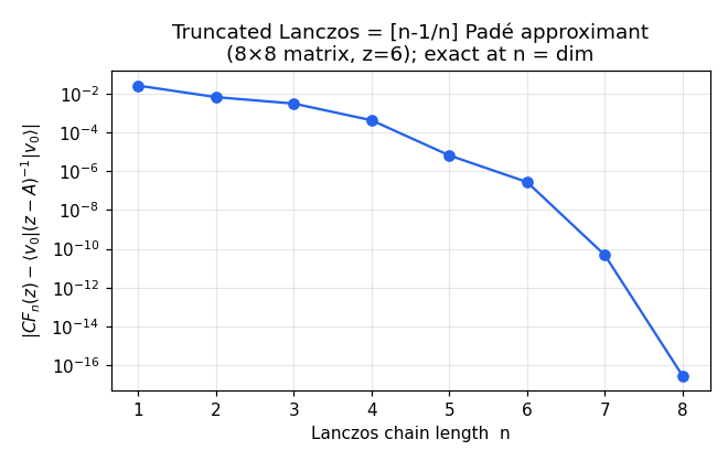

$Semilog plot of the error between the n-level continued fraction and the exact resolvent versus Lanczos chain length n, for an 8x8 matrix at z=6. The error falls roughly geometrically from about 0.026 at n=1 to machine precision (1e-17) at n=8.$

This is the content. Each truncated continued fraction $C F_{n}$ is a rational function of degree $n - 1$ over degree $n$ — the $[n - 1/ n]$ Padé approximant of the resolvent. Three Lanczos steps give a $[2/3]$ approximant already good to three digits; at $n = dim = 8$ it collapses onto the exact value at machine precision. Short chain, cheap approximation; full chain, exact. That is why you run a handful of Lanczos steps on a million-dimensional operator and read off a rational function instead of inverting anything — the 3×3-run-to-completion never shows you this, because it has no "short chain" to truncate.

3. Why $n$ Lanczos steps are the $[n - 1/ n]$ Padé approximant

The connection is the part that's genuinely hard to find stated plainly, so here it is in one chain of equalities. The resolvent is the moment-generating function of $v_{0}$ 's spectral measure $μ$ (the measure that puts weight $∣ ⟨ v_{0} ∣ ψ_{i} ⟩ ∣^{2}$ at each eigenvalue $λ_{i}$ of $A$ ):

G (z) = ⟨ v_{0} ∣ (z 1 - A)^{- 1} ∣ v_{0} ⟩ = \int \frac{d μ ( λ )}{z - λ} = k = 0 \sum \infty \frac{m _{k}}{z ^{k + 1}}, m_{k} = ⟨ v_{0} ∣ A^{k} ∣ v_{0} ⟩ .

The $m_{k}$ are the moments of $μ$ . Now three facts line up:

The $[n - 1/ n]$ Padé approximant of a power series is, by definition, the unique rational function (degree $n - 1$ over degree $n$ ) whose own series matches the first $2 n$ coefficients.
The $n$ -level Lanczos continued fraction is the Stieltjes transform of the $n$ -point Gauss quadrature rule for $μ$ — its nodes are the eigenvalues of the tridiagonal $T_{n}$ (the Ritz values), its weights the squared first components of $T_{n}$ 's eigenvectors.
$n$ -point Gauss quadrature is exact for polynomials up to degree $2 n - 1$ , so it reproduces the first $2 n$ moments $m_{0}, \dots, m_{2 n - 1}$ of $μ$ exactly.

Put them together: the $n$ -level Lanczos continued fraction is a degree- $(n - 1) / n$ rational function matching the first $2 n$ moments of $G (z)$ — which is exactly the $[n - 1/ n]$ Padé approximant. Lanczos coefficients = Gauss-quadrature rule = Padé approximant. Three names for one object, and the reason a 1950s numerical algorithm reproduces a 1890s moment-problem theorem.

Checked on the 8×8: at $n = 3$ the continued fraction reproduces the first $2 n = 6$ moments $m_{0}, \dots, m_{5}$ and first diverges from the truth at $m_{6}$ — the difference between $C F_{3} (z)$ and the six-moment sum $\sum_{k = 0}^{5} m_{k} / z^{k + 1}$ shrinks like $z^{- 7}$ as $z$ grows ( $1.3 \times 1 0^{- 9}$ at $z = 50$ , $8 \times 1 0^{- 14}$ at $z = 200$ ), precisely the "first unmatched moment is the 7th" signature of a six-moment match. The $[2/3]$ Padé is matching six moments, on the nose.

It's not a coincidence: the classical orthogonal polynomials are Lanczos

Everything above secretly lives in one classical theory — orthogonal polynomials on the real line. Recall the spectral measure $μ$ of $v_{0}$ (weight $∣ ⟨ v_{0} ∣ ψ_{i} ⟩ ∣^{2}$ at each eigenvalue). That measure has its own family of orthogonal polynomials ${p_{0}, p_{1}, p_{2}, \dots}$ , the ones obeying $\int p_{m} p_{n} d μ = δ_{mn}$ . Every such family satisfies a three-term recurrence,

x p_{n} (x) = β_{n} p_{n + 1} (x) + α_{n} p_{n} (x) + β_{n - 1} p_{n - 1} (x),

and the coefficients $(α_{n}, β_{n})$ of that recurrence are exactly the entries of the Jacobi (tridiagonal) matrix — which is to say, exactly what Lanczos hands back. So Lanczos is the algorithm that generates the orthogonal polynomials of $v_{0}$ 's spectral measure. The continued fraction is their Stieltjes transform, the Gauss quadrature is their roots-and-weights rule, the Padé approximant is their moment match. One structure, four names.

Which means the famous orthogonal polynomial families aren't separate objects to memorize — each is just Lanczos run on a classical weight. Take the multiplication-by- $x$ operator with weight $w (x)$ , start from $v_{0} = w$ , and the $α$ 's and $β$ 's that come out are the textbook recurrence coefficients:

# Run Lanczos on "multiply by x" with a classical weight w(x); out come the
# recurrence coefficients of THAT weight's orthogonal polynomials. The starting
# vector v0 = sqrt(weights) makes v0's spectral measure equal the weighted measure.
def recover(nodes, weights, m=6):
    return lanczos(nodes, np.sqrt(weights), m)

# Legendre: weight 1 on [-1,1]
x = np.linspace(-1, 1, 20000); a, b = recover(x, np.full(20000, 2/20000))
print("Legendre  beta:", b[:5], " vs  n/sqrt(4n^2-1)")
# Chebyshev (1st): weight 1/sqrt(1-x^2)
xc = np.cos((np.arange(4000)+0.5)*np.pi/4000); a, b = recover(xc, np.full(4000, np.pi/4000))
print("Chebyshev beta:", b[:5], " vs  1/sqrt2 then 1/2, 1/2, ...")
# Hermite: weight e^{-x^2}
xh, wh = np.polynomial.hermite.hermgauss(60); a, b = recover(xh, wh)
print("Hermite   beta:", b[:5], " vs  sqrt(n/2)")
# Laguerre: weight e^{-x} on [0, inf)
xl, wl = np.polynomial.laguerre.laggauss(60); a, b = recover(xl, wl)
print("Laguerre  alpha:", a[:5], " beta:", b[:5], " vs  2n+1  and  n")

Legendre  beta: [0.5774 0.5164 0.5071 0.5040 0.5025]   vs  n/sqrt(4n^2-1)
Chebyshev beta: [0.7071 0.5    0.5    0.5    0.5   ]   vs  1/sqrt2 then 1/2, 1/2, ...
Hermite   beta: [0.7071 1.     1.2247 1.4142 1.5811]   vs  sqrt(n/2)
Laguerre  alpha: [1. 3. 5. 7. 9.]  beta: [1. 2. 3. 4. 5.]   vs  2n+1  and  n

Every one matches its textbook formula — Legendre's $β_{n} = n / 4 n^{2} - 1$ , Chebyshev's $(1/ 2, \frac{1}{2}, \frac{1}{2}, \dots)$ , Hermite's $n /2$ , Laguerre's diagonal $2 n + 1$ and off-diagonal $n$ — recovered by running the same Lanczos routine from the top of this page on the right measure. The classical families are the special cases where the measure happens to be a classical weight; the named Gauss quadratures are the same Jacobi-matrix eigenproblem (Golub-Welsch):

family	weight $w (x)$	interval	Jacobi off-diagonals $β_{n}$	quadrature
Legendre	$1$	$[- 1, 1]$	$n / 4 n^{2} - 1$	Gauss-Legendre
Chebyshev (1st)	$(1 - x^{2})^{- 1/2}$	$[- 1, 1]$	$1/ 2, \frac{1}{2}, \frac{1}{2}, \dots$	Gauss-Chebyshev
Hermite	$e^{- x^{2}}$	$(- \infty, \infty)$	$n /2$	Gauss-Hermite
Laguerre	$e^{- x}$	$[0, \infty)$	$n$ (diag $2 n + 1$ )	Gauss-Laguerre
Jacobi	$(1 - x)^{a} (1 + x)^{b}$	$[- 1, 1]$	(closed form in $a, b$ )	Gauss-Jacobi

Watch the matrix collapse to tridiagonal

The recovery above runs Lanczos and reads off the $β$ 's. But you can see why the matrix is tridiagonal in the first place without running Lanczos at all. Build the orthonormal polynomials of a weight by plain Gram-Schmidt, then fill in the multiplication-by- $x$ matrix $M_{ij} = ⟨ \tilde{p}_{i}, x \tilde{p}_{j} ⟩$ by quadrature — using none of the recurrence coefficients, so the structure is an output. Every entry more than one step off the diagonal comes back as machine zero. Pick a column to see what multiplication by $x$ does to a single basis polynomial: it can only reach one degree up, and self-adjointness kills everything more than one degree down.

Build the orthonormal polynomials of the Legendre weight by Gram–Schmidt, then fill the matrix M[i][j] = ⟨P̃ᵢ, x·P̃ⱼ⟩ by quadrature — no recurrence coefficients used. Click a column to see what multiplying by x does to that basis polynomial.

columns j → ; rows i ↓ (basis index 0…6)

x · P̃₂ = (decomposition onto the basis)

P̃₀

≈0

P̃₁

0.516

P̃₂

≈0

P̃₃

0.507

P̃₄

≈0

P̃₅

≈0

P̃₆

≈0

Only P̃₁, P̃₂ and P̃₃ survive. Multiplying by x raises the degree to 3 (so nothing above P̃₃), and orthogonality kills everything below P̃₁: ⟨x·P̃₂, P̃_m⟩ = ⟨P̃₂, x·P̃_m⟩, and x·P̃_m has degree m+1 < 2 whenever m < 1. Three terms, forced.

Everything more than one step off the diagonal came out ≈0 (≤ 10⁻¹³, the quadrature floor) — computed, not assumed. The off-diagonal band you do see is the Lanczos β sequence: for Legendre that's the textbook recurrence coefficient. Symmetric, because multiplication by the real variable x is self-adjoint; tridiagonal, because x raises degree by exactly one. Run Lanczos on this measure and these same numbers fall out.

Two facts are doing all the work. Multiplication by $x$ is self-adjoint — $⟨ x f, g ⟩ = ⟨ f, xg ⟩$ , because $x$ is real and slides across the integral with no conjugate — so $M$ is symmetric. And $x \tilde{p}_{j}$ has degree $j + 1$ , so it is orthogonal to every $\tilde{p}_{i}$ with $i > j + 1$ ; symmetry then forces the mirror zeros below $i < j - 1$ . A symmetric matrix that vanishes outside the first off-diagonal is exactly a tridiagonal one — a three-term recurrence. The Jacobi matrix isn't a lucky shape; it's the only shape these two facts allow.

The converse closes the loop. Favard's theorem (1935): any sequence obeying that three-term recurrence with real $β_{n} > 0$ is the orthogonal-polynomial family of some positive measure. So the correspondence is a clean bijection,

{Jacobi matrices, β_{n} > 0} ⟷ {positive measures} ⟷ {orthogonal-polynomial families},

and Lanczos is the constructive direction: hand it an operator and a vector, it builds the Jacobi matrix, which is a measure's orthogonal polynomials. Run it on a textbook weight and you get Legendre or Hermite; run it on a quantum Hamiltonian and a state, you get the bespoke orthogonal polynomials of that system's spectral density — and their continued fraction is the resolvent, their Gauss rule is the spectral-density approximation, their Padé is the moment match. Stieltjes (1894), Favard (1935), Gauss quadrature, Lanczos (1950), and the continued fraction at the top of this page are all the same theorem about the same object. Not a coincidence — just the moment problem, seen from five directions.

Related on this site

Lanczos iteration — the algorithm that produces the α's and β's.
Padé via Lanczos — the same correspondence put to work in model-order reduction.
Padé approximants — what [m/n] means and where it comes from.
Legendre polynomials — one of the classical families that falls out of Lanczos on a flat weight.
Chebyshev nodes — Gauss-Chebyshev quadrature, the same Jacobi-matrix eigenproblem.
Obara-Saika — the same three-term recurrence in quantum chemistry: the Gaussian-integral angular-momentum ladder is the Hermite recurrence.