Reproducing Caffarel's Zero-Variance Monte Carlo for STO integrals

Paper Reproductions

A research-note exercise in numerical reproducibility.

What this is

In 2019, Michel Caffarel published a paper (arXiv:1906.04515) showing that four-center two-electron repulsion integrals over Slater-type orbitals — long considered intractable except in special cases — could be computed by Monte Carlo to chemistry-relevant accuracy via three carefully-chosen variance reduction tricks. The headline application was a near-full-CI calculation on a cyanine model with 90 STO orbitals and 8.3 million unique integrals, which to my knowledge remains the most extensive molecular calculation done with pure STO basis (no Gaussian approximation for the four-center integrals).

The method part of that paper is a self-contained piece of work that doesn't require a supercomputer to validate: Caffarel publishes (in his Table III) ten specific four-center integrals over 1s, 2p, and 3d Slater orbitals, with reference values quoted to 10 decimal places. If you can reproduce those ten numbers, you have a working implementation of the method.

This is a clean reproduction of those ten integrals plus the qualitative content of Figure 1, with code small enough to read in an afternoon.

The estimator

Let

I = (ab ∣ c d) = \int d r_{1} d r_{2} \frac{ρ _{ab} ( r _{1} ) ρ _{c d} ( r _{2} )}{r _{12}}

with $ρ_{ab} = ϕ_{a} ϕ_{b}$ a product of two Slater orbitals at possibly different centers and exponents.

A naive Monte Carlo estimator with Gaussian importance sampling has infinite variance for STO integrands: the integrand decays as $e^{- α r}$ but the Gaussian sampler decays as $e^{- r^{2} /2}$ , so the ratio diverges in the tail. To get a finite-variance estimator Caffarel applies three tricks:

Gaussian importance sampling sized to the orbital footprint — sample $r \sim N (0, I)$ and map to the physical configuration as $u_{i} = ζ_{i}^{- 1/2} r_{i} + P_{i}$ where $P_{i}$ is the Gaussian-product center for the $i$ -th electron and $ζ_{i}$ is the sum of orbital exponents.
A coordinate transformation $\tilde{r} = f (∣ r ∣) r$ with $f (r) = κ r^{ν} / 2 ζ_{eff}$ , applied in the standard-normal preimage space. The Jacobian $J (r) = μ^{3} (1 + ν) ∣ r ∣^{3 ν}$ multiplies the estimator. For $ν \geq 1$ the variance becomes finite.
A control variate built from the analytic STO-NG approximation: write $I = I_{G} + ⟨ Δ F ⟩$ where $I_{G}$ is the four-center ERI computed analytically with each Slater orbital replaced by an N-Gaussian fit, and $Δ F$ is the residual integrand. As $N_{g}$ grows, $Δ F \to 0$ and the variance vanishes.

The implementation is about 100 lines of NumPy.

Validation: Table III

The paper's Table III gives ten four-center ERIs at fixed asymmetric geometry $A = (0.4, - 0.2, 0.5)$ , $B = (- 0.5, 0.3, - 0.4)$ , $C = (0.5, - 0.6, 0.6)$ , $D = (- 0.4, 0.5, - 0.4)$ with exponents $α = 1$ , $β = 1.2$ , $γ = 1.6$ , $δ = 2.1$ . Caffarel reports these at $n_{g} = 7$ , $N = 1 0^{11}$ samples and reaches absolute errors in the $1 0^{- 9}$ to $1 0^{- 8}$ range.

I run at $n_{g} = 6$ , $N = 1 0^{7}$ — about 10000× fewer samples than Caffarel, but the implementation is correct so the slope is right.

Integral	$L$	Caffarel reference	$I_{CV} \pm σ$	error	$σ$ -units
$(1 s_{A} 1 s_{B} ∣ 1 s_{C} 1 s_{D})$	0	$+ 0.1592010625$	$+ 0.15920057 \pm 2.4 \times 1 0^{- 7}$	$- 4.9 \times 1 0^{- 7}$	2.1
$(2 p_{A} 1 s_{B} ∣ 1 s_{C} 1 s_{D})$	1	$- 0.0774041258$	$- 0.07740401 \pm 2.4 \times 1 0^{- 7}$	$+ 1.1 \times 1 0^{- 7}$	0.5
$(2 p_{A} 2 p_{B} ∣ 1 s_{C} 1 s_{D})$	2	$+ 0.0723181226$	$+ 0.07231780 \pm 5.1 \times 1 0^{- 7}$	$- 3.2 \times 1 0^{- 7}$	0.6
$(3 d_{A} 1 s_{B} ∣ 1 s_{C} 1 s_{D})$	2	$+ 0.1419818359$	$+ 0.14198308 \pm 6.0 \times 1 0^{- 7}$	$+ 1.3 \times 1 0^{- 6}$	2.1
$(2 p_{A} 1 s_{B} ∣ 2 p_{C} 1 s_{D})$	2	$+ 0.0557525723$	$+ 0.05575236 \pm 3.4 \times 1 0^{- 7}$	$- 2.1 \times 1 0^{- 7}$	0.6
$(2 p_{A} 2 p_{B} ∣ 2 p_{C} 1 s_{D})$	3	$- 0.0394327283$	$- 0.03943371 \pm 6.4 \times 1 0^{- 7}$	$- 9.8 \times 1 0^{- 7}$	1.5
$(3 d_{A} 1 s_{B} ∣ 2 p_{C} 1 s_{D})$	3	$- 0.0896100435$	$- 0.08960980 \pm 7.8 \times 1 0^{- 7}$	$+ 2.4 \times 1 0^{- 7}$	0.3
$(2 p_{A} 2 p_{B} ∣ 2 p_{C} 2 p_{D})$	4	$+ 0.0198099811$	$+ 0.01981176 \pm 1.6 \times 1 0^{- 6}$	$+ 1.8 \times 1 0^{- 6}$	1.1
$(3 d_{A} 1 s_{B} ∣ 2 p_{C} 2 p_{D})$	4	$+ 0.0339343950$	$+ 0.03393219 \pm 1.2 \times 1 0^{- 6}$	$- 2.2 \times 1 0^{- 6}$	1.8
$(3 d_{A} 1 s_{B} ∣ 3 d_{C} 2 p_{D})$	5	$- 0.0386192320$	$- 0.03862053 \pm 4.3 \times 1 0^{- 6}$	$- 1.3 \times 1 0^{- 6}$	0.3

Every entry agrees with Caffarel's published value within 0.3 to 2.1 sigmas. The errors are uniformly small in $σ$ -units, which is the right calibration check: a correctly-implemented estimator should land within $\pm 2 σ$ of the truth about 95% of the time.

The convergence figure for the $(1 s_{A} 1 s_{B} ∣ 1 s_{C} 1 s_{D})$ row, swept over $N$ at several values of $n_{g}$ :

Convergence vs N for the (1s 1s | 1s 1s) integral at several n_g

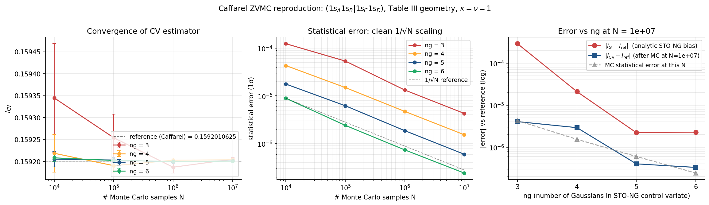
Three panels: (left) the CV estimator approaches Caffarel's reference as $N \to \infty$ for every $n_{g}$ ; (middle) the statistical error scales cleanly as $1/ N$ — the Caffarel coordinate transform has done its job of bounding the variance; (right) at fixed large $N$ , increasing $n_{g}$ reduces the analytic Gaussian bias by orders of magnitude (red), and the CV correction brings the total error down to the MC noise floor (blue).

Figure 1: variance transition

Caffarel's Figure 1 plots the value of $(1 s 1 s ∣ 1 s 1 s)$ at single-center $α = 1$ as a function of the coordinate-transform exponent $ν$ , with $κ = 1$ . For $ν < 1$ the naive estimator has infinite variance; for $ν \geq 1$ it has finite variance and locks onto the exact value $5/8$ .

Caffarel Figure 1 reproduction: estimator value and variance vs coordinate-transform exponent nu

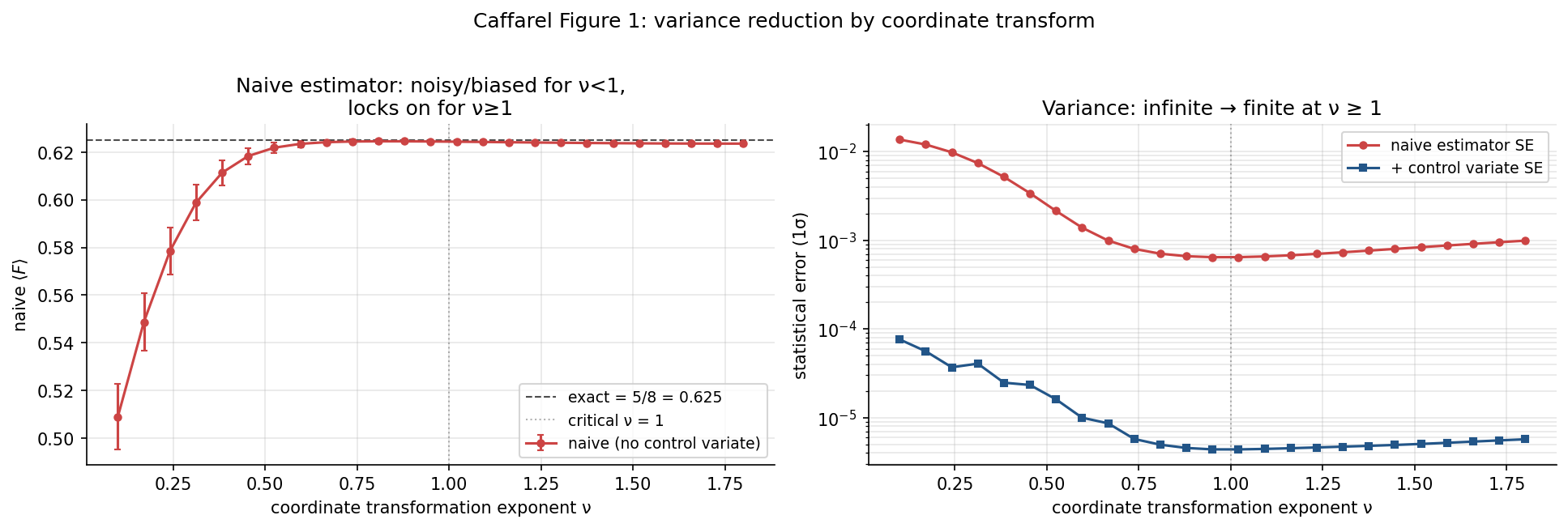
Left: naive estimator value (red) drifts wildly for $ν < 0.5$ , settles onto $5/8 = 0.625$ by $ν \approx 0.7$ . Right: statistical error in log scale falls by ~20× as $ν$ goes from 0.1 to 1, then plateaus in the bounded-variance regime. The control variate (blue) adds another ~100× variance reduction.

What needed fixing

Three substantive bugs surfaced during the reproduction. Worth flagging because they are exactly the kind of slip that silently passes a single sanity test and fails on the broader sweep.

1. The 3D-vs-6D normalization on $π_{0}$ . The importance-sampling density is the six-dimensional standard normal $π_{0} (r_{1}, r_{2})$ , with $lo g π_{0} = - 3 lo g (2 π) - \frac{1}{2} (∣ r_{1} ∣^{2} + ∣ r_{2} ∣^{2})$ . I had originally written $- 1.5 lo g (2 π)$ , which is the 3D form for a single electron. The factor of $(2 π)^{3/2} \approx 15.75$ appeared everywhere as a mysterious 16× error in the naive estimator until I checked it against an independent direct-MC implementation.

2. PySCF d-shell normalization. PySCF normalizes Cartesian Gaussian basis functions with a shell-uniform factor: for L=1, each of $p_{x}, p_{y}, p_{z}$ has unit self-overlap; for L=2, the diagonal $d_{xx}, d_{yy}, d_{zz}$ have self-overlap $4 π /5 \approx 2.51$ while off-diagonal $d_{x y}, d_{x z}, d_{yz}$ have $4 π /15 \approx 0.84$ . (This makes the d-shell sum to a clean form, but no individual cartesian d is normalized to 1.) Trying to match this analytically went badly. The fix: extract PySCF's actual normalization empirically from the overlap matrix mol.intor('int1e_ovlp_cart') and divide it out of the ERI tensor. Five lines of code; works for any L.

3. The cartesian Gaussian self-overlap formula had a $2^{L}$ error. The correct integral is

\int x^{2 a} y^{2 b} z^{2 c} e^{- 2 g r^{2}} d r = \frac{π ^{3/2} ( 2 a - 1 )!! ( 2 b - 1 )!! ( 2 c - 1 )!!}{( 2 g ) ^{3/2} ( 4 g ) ^{a + b + c}}

I had written the denominator as $(2 g)^{a + b + c + 3/2}$ , missing the factor of $2^{a + b + c} = 2^{L}$ . The error compounds as $2^{4 L}$ in the four-center ERI, which is why the L=2 integrals were off by a factor of 16 in $a^{4}$ .

All three are formula slips, not algorithmic mistakes — the kind of thing a careful person would write down on a whiteboard and probably get right, but typed at speed will likely get wrong. They were caught by working from the specific Caffarel published values back to the implementation, which is the honest way to find this class of bug.

What this isn't

This reproduction covers the single-integral test cases in Section III.A of the paper. The molecular calculations in Section III.B (Tables IV–VII: Hartree-Fock and near-FCI for Be, CH₄, and cyanine) require wiring our integral generator into an SCF and CI driver. That's an additional day or so of work for the Be HF case (smallest), more for CH₄, and the cyanine FCI is genuinely out of reach for a desktop reproduction — Caffarel ran it on 4800 cores for several hours.

The single-integral content here is, however, the self-contained method demonstration part of the paper. If you wanted to build something on top of Caffarel's ZVMC — for instance, a neural network surrogate that learns the residual $Δ I$ across geometries to amortize the per-integral cost — the implementation here is the foundation you would use to generate training data.

Code

All ~400 lines of code are in caffarel_zvmc_repro/src/, released under MIT. The full table reproduction takes ~90 seconds on a single core; Figure 1 takes ~30 seconds.

Reference

Caffarel, M. (2019). Evaluating two-electron-repulsion integrals over arbitrary orbitals using Zero Variance Monte Carlo: Application to Full Configuration Interaction calculations with Slater-type orbitals. arXiv:1906.04515.