Chebyshev Polynomial Root Distribution

Spectral Methods

This page explores the distribution of roots of random Chebyshev polynomials, comparing unconstrained coefficients with coefficients constrained to lie on a hypersphere.

Chebyshev Polynomials

Chebyshev polynomials of the first kind are defined by the recurrence relation:

T_{0} (x) = 1, T_{1} (x) = x, T_{n + 1} (x) = 2 x T_{n} (x) - T_{n - 1} (x)

A random Chebyshev polynomial of degree $n$ can be constructed as:

P (x) = k = 0 \sum n c_{k} T_{k} (x)

where $c_{k}$ are random coefficients.

Constrained vs Unconstrained

We compare two ensembles:

Unconstrained: $c_{k} \sim N (0, 1)$ (standard normal)
Hypersphere: $c$ normalized to lie on a hypersphere of radius $R$

The root distribution shows interesting concentration properties near the unit circle.

Implementation

The following code samples roots from both ensembles and analyzes their distribution:

import numpy as np
import matplotlib.pyplot as plt
import matplotlib as mpl

def set_publication_style():
    """Set publication-quality matplotlib style."""
    mpl.rcParams.update({
        'font.family': 'serif',
        'font.size': 12,
        'axes.labelsize': 14,
        'axes.titlesize': 16,
        'axes.linewidth': 1.2,
        'axes.labelpad': 8,
        'axes.titlepad': 10,
        'xtick.labelsize': 12,
        'ytick.labelsize': 12,
        'xtick.direction': 'in',
        'ytick.direction': 'in',
        'xtick.top': True,
        'ytick.right': True,
        'xtick.major.size': 6,
        'ytick.major.size': 6,
        'xtick.major.width': 1.2,
        'ytick.major.width': 1.2,
        'legend.fontsize': 12,
        'legend.frameon': False,
        'lines.linewidth': 2,
        'lines.markersize': 6,
        'figure.dpi': 100,
        'savefig.dpi': 300,
        'savefig.bbox': 'tight'
    })

set_publication_style()
from numpy.polynomial import Chebyshev, Polynomial

# ---------------- PARAMETERS ----------------
degree = 50
num_polys = 400
radius = 1.0
seed = 0

np.random.seed(seed)

# ---------------- CHEBYSHEV GENERATORS ----------------
def cheb_unconstrained(n):
    return np.random.randn(n + 1)

def cheb_on_sphere(n, R=1.0):
    c = np.random.randn(n + 1)
    return c * (R / np.linalg.norm(c))

# ---------------- SAMPLE ROOTS ----------------
def sample_roots_cheb(gen):
    roots = []
    for _ in range(num_polys):
        c = gen(degree)

        # Chebyshev polynomial → monomial polynomial
        T = Chebyshev(c)
        P = T.convert(kind=Polynomial)

        roots.append(P.roots())
    return np.concatenate(roots)

roots_un = sample_roots_cheb(cheb_unconstrained)
roots_con = sample_roots_cheb(cheb_on_sphere)

# ---------------- RADIAL DATA ----------------
du = np.abs(roots_un) - 1.0
dc = np.abs(roots_con) - 1.0

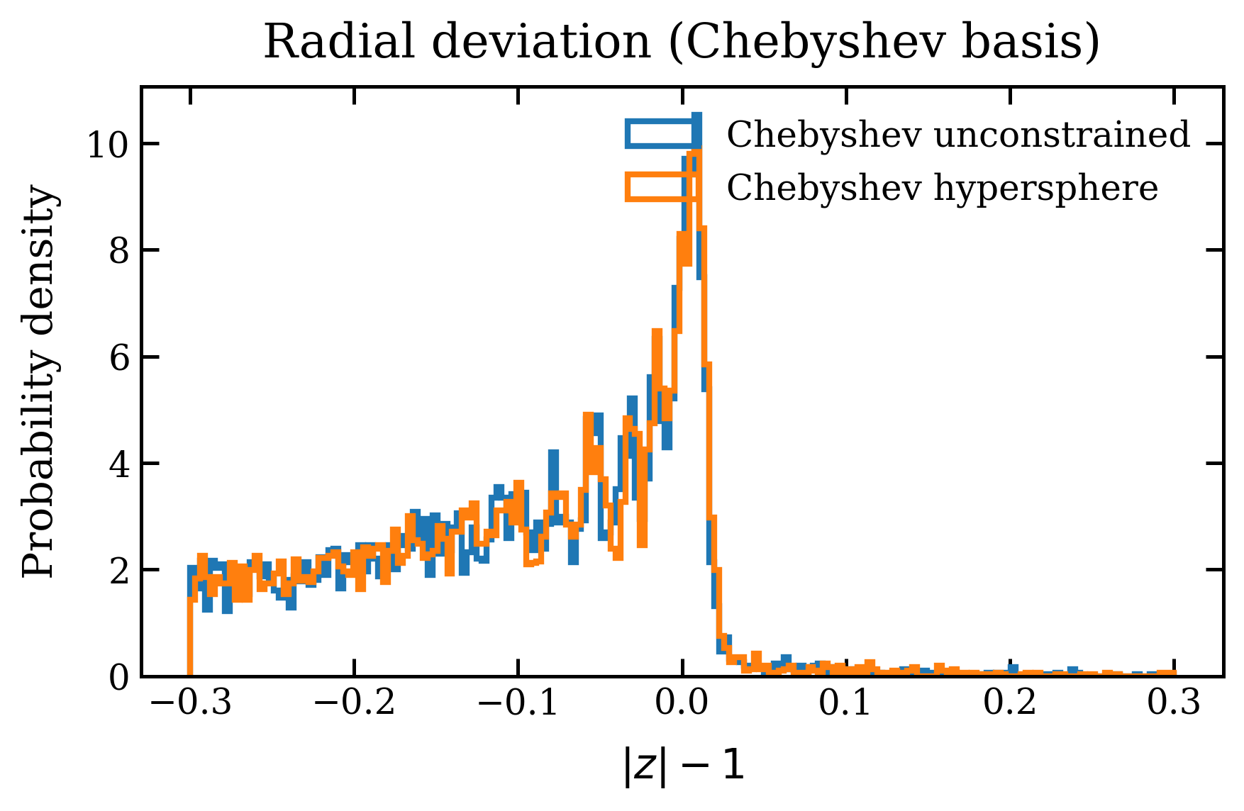
# ---------------- PDF OF r - 1 ----------------
bins = np.linspace(-0.3, 0.3, 200)

plt.figure(figsize=(6,4))
plt.hist(du, bins=bins, density=True, histtype="step",
         linewidth=2, label="Chebyshev unconstrained")
plt.hist(dc, bins=bins, density=True, histtype="step",
         linewidth=2, label="Chebyshev hypersphere")
plt.xlabel(r"$|z| - 1$")
plt.ylabel("Probability density")
plt.title("Radial deviation (Chebyshev basis)")
plt.legend()
plt.tight_layout()
plt.savefig('figures/chebyshev_roots_pdf.png', dpi=300, bbox_inches='tight')
plt.show()

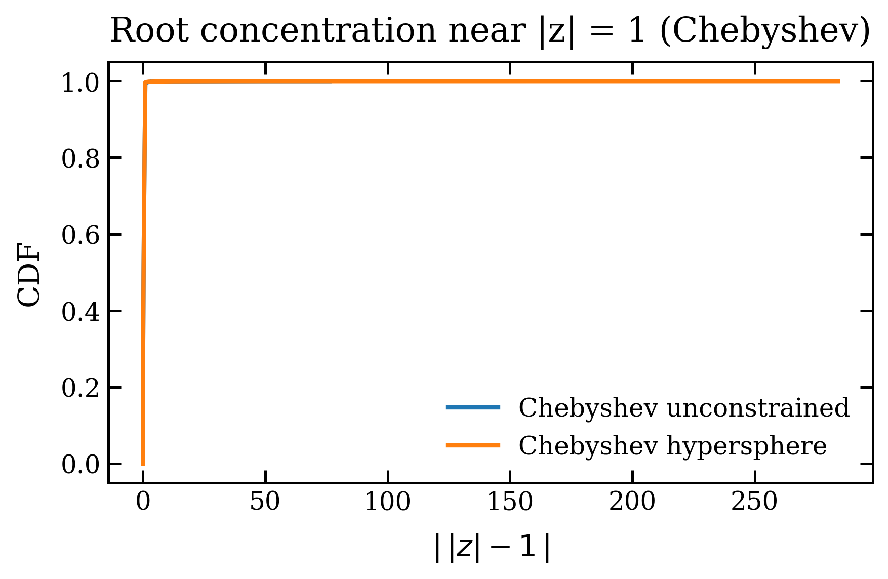
# ---------------- CDF OF |r - 1| ----------------
xu = np.sort(np.abs(du))
xc = np.sort(np.abs(dc))

Fu = np.arange(1, len(xu)+1) / len(xu)
Fc = np.arange(1, len(xc)+1) / len(xc)

plt.figure(figsize=(6,4))
plt.plot(xu, Fu, linewidth=2, label="Chebyshev unconstrained")
plt.plot(xc, Fc, linewidth=2, label="Chebyshev hypersphere")
plt.xlabel(r"$|\,|z| - 1\,|$")
plt.ylabel("CDF")
plt.title("Root concentration near |z| = 1 (Chebyshev)")
plt.legend()
plt.tight_layout()
plt.savefig('figures/chebyshev_roots_cdf.png', dpi=300, bbox_inches='tight')
plt.show()

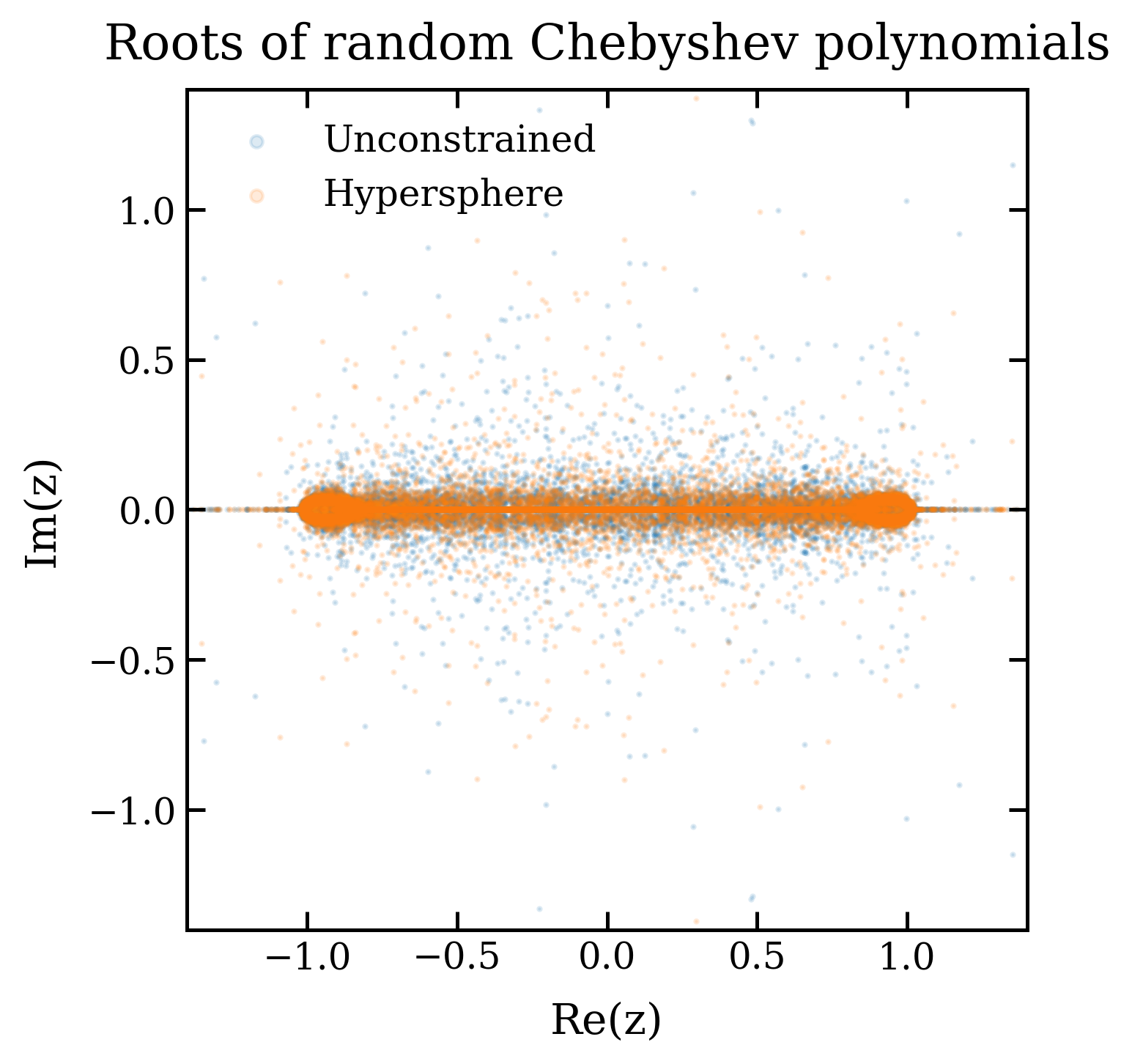
# ---------------- COMPLEX PLANE (ZOOMED) ----------------
Rmax = 1.4

plt.figure(figsize=(5,5))
plt.scatter(roots_un.real, roots_un.imag,
            s=1, alpha=0.15, label="Unconstrained")
plt.scatter(roots_con.real, roots_con.imag,
            s=1, alpha=0.15, label="Hypersphere")
plt.gca().set_aspect("equal")
plt.xlim(-Rmax, Rmax)
plt.ylim(-Rmax, Rmax)
plt.xlabel("Re(z)")
plt.ylabel("Im(z)")
plt.title("Roots of random Chebyshev polynomials")
plt.legend(markerscale=4)
plt.tight_layout()
plt.savefig('figures/chebyshev_roots_complex.png', dpi=300, bbox_inches='tight')
plt.show()

# ---------------- NUMERICAL SUMMARY ----------------
print("Std(|r-1|) for Chebyshev ensemble:")
print("  Unconstrained :", np.std(du))
print("  Hypersphere   :", np.std(dc))

Visualization

The following plots show the distribution of Chebyshev polynomial roots:

Key Observations

Roots of random Chebyshev polynomials tend to cluster near the unit circle
Constraining coefficients to a hypersphere affects the root distribution
The standard deviation of $∣ r ∣ - 1$ provides a measure of root concentration
Visualization in the complex plane reveals the distribution pattern