Chebyshev Collocation Method

import numpy as np
import scipy.linalg
import scipy.integrate
import matplotlib.pyplot as plt

def set_publication_style():
    """Set publication-quality matplotlib style."""
    plt.rcParams.update({
        'font.family': 'serif',
        'font.size': 12,
        'axes.labelsize': 14,
        'axes.titlesize': 16,
        'axes.linewidth': 1.2,
        'axes.labelpad': 8,
        'axes.titlepad': 10,
        'xtick.labelsize': 12,
        'ytick.labelsize': 12,
        'xtick.direction': 'in',
        'ytick.direction': 'in',
        'xtick.top': True,
        'ytick.right': True,
        'xtick.major.size': 6,
        'ytick.major.size': 6,
        'xtick.major.width': 1.2,
        'ytick.major.width': 1.2,
        'legend.fontsize': 12,
        'legend.frameon': False,
        'lines.linewidth': 2,
        'lines.markersize': 6,
        'figure.dpi': 100,
        'savefig.dpi': 300,
        'savefig.bbox': 'tight'
    })

set_publication_style()

# Compute Chebyshev-Lobatto points
def chebyshev_points(N):
    return np.cos(np.pi * np.arange(N) / (N - 1))

# Compute Chebyshev differentiation matrix
def chebyshev_diff_matrix(N, x):
    D = np.zeros((N, N))
    c = np.array([2] + [1] * (N - 2) + [2]) * (-1) ** np.arange(N)
    
    for i in range(N):
        for j in range(N):
            if i != j:
                D[i, j] = c[i] / (c[j] * (x[i] - x[j]))
        D[i, i] = -np.sum(D[i, :])
    
    return D

# Gaussian elimination with partial pivoting
def gaussian_elimination(A, b):
    N = len(b)
    for k in range(N):
        # Pivot
        max_row = np.argmax(np.abs(A[k:, k])) + k
        A[[k, max_row]] = A[[max_row, k]]
        b[[k, max_row]] = b[[max_row, k]]
        
        # Eliminate
        for i in range(k + 1, N):
            factor = A[i, k] / A[k, k]
            A[i, k:] -= factor * A[k, k:]
            b[i] -= factor * b[k]
    
    # Back-substitution
    x = np.zeros(N)
    for i in range(N - 1, -1, -1):
        x[i] = (b[i] - np.dot(A[i, i+1:], x[i+1:])) / A[i, i]
    
    return x

# Solve BVP using Chebyshev collocation method
def solve_bvp(N):
    x = chebyshev_points(N)
    D = chebyshev_diff_matrix(N, x)
    D2 = np.dot(D, D)  # Second derivative matrix
    
    # Construct the system: D2 * y - y = f
    A = D2 - np.eye(N)
    f = np.sin(np.pi * x)
    
    # Apply boundary conditions: y(-1) = 0, y(1) = 0
    A = A[1:-1, 1:-1]  # Remove first and last rows/columns
    f = f[1:-1]  # Remove first and last values
    
    # Solve using Gaussian elimination
    y_inner = gaussian_elimination(A, f)
    
    # Construct the full solution with boundary conditions
    y = np.zeros(N)
    y[1:-1] = y_inner
    return x, y

# Solve BVP using scipy solver
def solve_bvp_scipy():
    def ode_fun(x, y):
        return [y[1], y[0] + np.sin(np.pi * x)]
    
    def bc(ya, yb):
        return [ya[0], yb[0]]
    
    x_mesh = np.linspace(-1, 1, 100)
    y_guess = np.zeros((2, x_mesh.size))
    sol = scipy.integrate.solve_bvp(ode_fun, bc, x_mesh, y_guess)
    return sol.x, sol.y[0]

# Run for N=16 points
N = 16
x, y = solve_bvp(N)
x_scipy, y_scipy = solve_bvp_scipy()

# Plot result
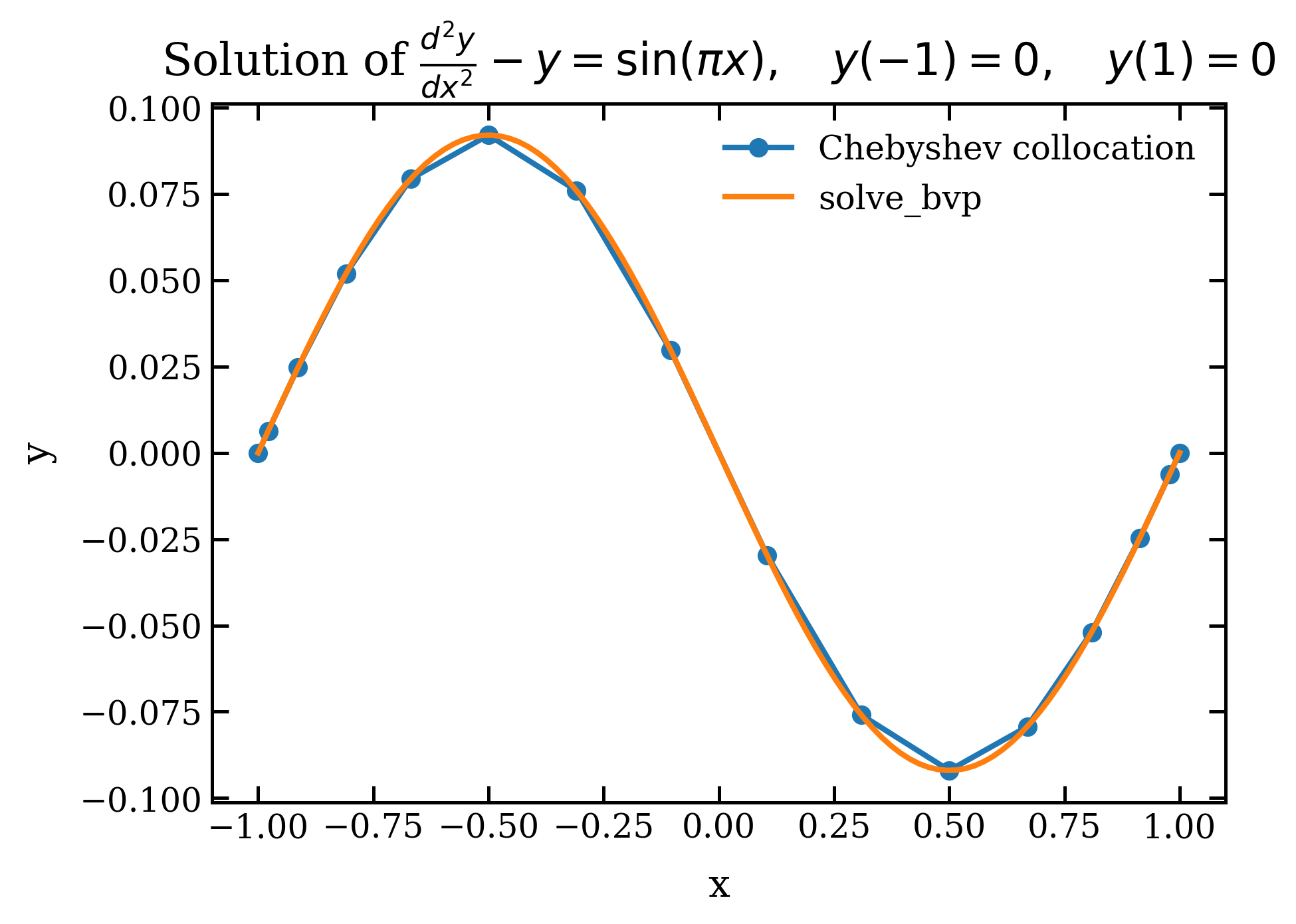
plt.title(r"Solution of $\frac{d^2 y}{dx^2} - y = \sin(\pi x), \quad y(-1) = 0, \quad y(1) = 0$")
plt.plot(x, y, 'o-', label='Chebyshev collocation')
plt.plot(x_scipy, y_scipy, '-', label='solve_bvp')
plt.xlabel('x')
plt.ylabel('y')
plt.legend()
plt.tight_layout()  # Automatically adjusts layout
plt.savefig('figures/chebyshev_collocation_solution.png', dpi=300, bbox_inches='tight')
plt.show()