Spectral Derivative

Spectral Methods

Spectral methods compute derivatives using the Fourier transform, providing extremely high accuracy for smooth, periodic functions. The method transforms the function to frequency space, multiplies by the wavenumber, and transforms back.

Mathematical Formulation

For a function $f (x)$ on a periodic domain, the derivative can be computed using the Fourier transform:

\frac{df}{d x} = F^{- 1} [ik F [f]]

where $F$ is the Fourier transform, $F^{- 1}$ is the inverse Fourier transform, and $k$ is the wavenumber.

In discrete form, for a function sampled at $N$ points with spacing $Δ x$ :

k_{j} = \frac{2 πj}{N Δ x}, j = - \frac{N}{2}, \dots, \frac{N}{2} - 1

The derivative is computed as:

\frac{df}{d x}_{j} = Re [IFFT (i k_{j} \cdot FFT (f_{j}))]

Accuracy

Spectral differentiation provides exponential convergence for smooth, periodic functions. For a function with $p$ continuous derivatives, the error scales as $O (N^{- p})$ , where $N$ is the number of grid points.

This is far superior to finite difference methods, which typically provide only polynomial convergence (e.g., $O (h^{2})$ for centered differences).

Python Implementation

The following code implements spectral differentiation using FFT:

import numpy as np
import matplotlib.pyplot as plt
import matplotlib as mpl

def set_publication_style():
    """Set publication-quality matplotlib style."""
    mpl.rcParams.update({
        'font.family': 'serif',
        'font.size': 12,
        'axes.labelsize': 14,
        'axes.titlesize': 16,
        'axes.linewidth': 1.2,
        'axes.labelpad': 8,
        'axes.titlepad': 10,
        'xtick.labelsize': 12,
        'ytick.labelsize': 12,
        'xtick.direction': 'in',
        'ytick.direction': 'in',
        'xtick.top': True,
        'ytick.right': True,
        'xtick.major.size': 6,
        'ytick.major.size': 6,
        'xtick.major.width': 1.2,
        'ytick.major.width': 1.2,
        'legend.fontsize': 12,
        'legend.frameon': False,
        'lines.linewidth': 2,
        'lines.markersize': 6,
        'figure.dpi': 100,
        'savefig.dpi': 300,
        'savefig.bbox': 'tight'
    })

set_publication_style()

def spectral_derivative(f, x):
    """
    Compute the derivative of a function using spectral methods (FFT).
    
    Parameters:
    -----------
    f : array
        Function values on a periodic grid
    x : array
        Grid points (must be uniformly spaced)
    
    Returns:
    --------
    df_dx : array
        Derivative values at grid points
    """
    N = len(f)
    dx = x[1] - x[0]  # Grid spacing
    
    # Compute FFT
    f_hat = np.fft.fft(f)
    
    # Compute wavenumbers
    k = 2 * np.pi * np.fft.fftfreq(N, d=dx)
    
    # Apply derivative operator in frequency space
    df_hat = 1j * k * f_hat
    
    # Transform back to physical space
    df_dx = np.fft.ifft(df_hat).real
    
    return df_dx

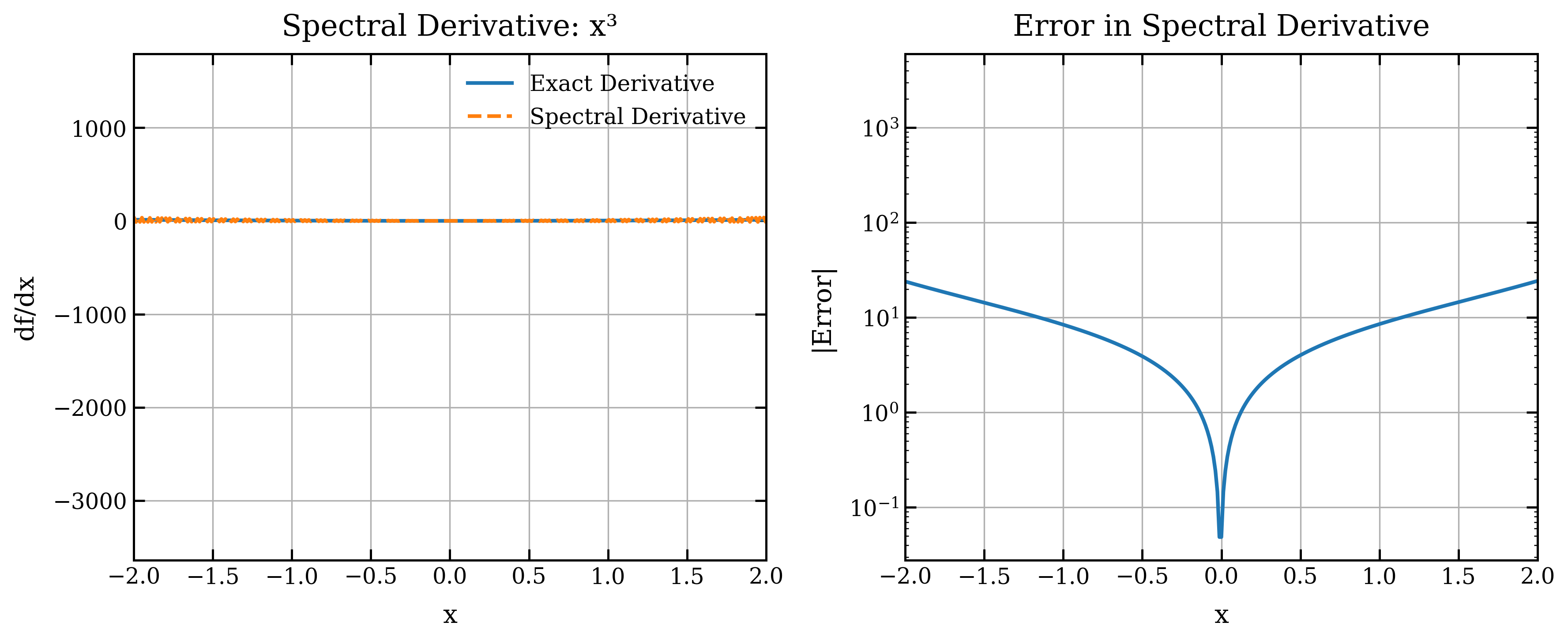
# Example 1: Polynomial function
N = 500
L = 2 * np.pi
x = np.linspace(-L/2, L/2, N, endpoint=False)
f = x**3
exact_derivative = 3 * x**2

df_spectral = spectral_derivative(f, x)

# Plot results
plt.figure(figsize=(12, 5))

plt.subplot(1, 2, 1)
plt.plot(x, exact_derivative, label="Exact Derivative", linewidth=2)
plt.plot(x, df_spectral, '--', label="Spectral Derivative", linewidth=2)
plt.xlabel("x")
plt.ylabel("df/dx")
plt.title("Spectral Derivative: x³")
plt.legend()
plt.grid(True)
plt.xlim(-2, 2)

plt.subplot(1, 2, 2)
error = np.abs(df_spectral - exact_derivative)
plt.semilogy(x, error, linewidth=2)
plt.xlabel("x")
plt.ylabel("|Error|")
plt.title("Error in Spectral Derivative")
plt.grid(True)
plt.xlim(-2, 2)

plt.tight_layout()
plt.savefig('figures/spectral_derivative_comparison.png', dpi=300, bbox_inches='tight')
plt.show()

print(f"Maximum error: {np.max(error):.2e}")
print(f"Mean error: {np.mean(error):.2e}")

# Example 2: Smooth periodic function (better suited for spectral methods)
x2 = np.linspace(0, 2*np.pi, N, endpoint=False)
f2 = np.sin(x2) * np.cos(2*x2)
exact_derivative2 = np.cos(x2) * np.cos(2*x2) - 2 * np.sin(x2) * np.sin(2*x2)

df_spectral2 = spectral_derivative(f2, x2)

plt.figure(figsize=(12, 5))

plt.subplot(1, 2, 1)
plt.plot(x2, exact_derivative2, label="Exact Derivative", linewidth=2)
plt.plot(x2, df_spectral2, '--', label="Spectral Derivative", linewidth=2)
plt.xlabel("x")
plt.ylabel("df/dx")
plt.title("Spectral Derivative: sin(x)cos(2x)")
plt.legend()
plt.grid(True)

plt.subplot(1, 2, 2)
error2 = np.abs(df_spectral2 - exact_derivative2)
plt.semilogy(x2, error2, linewidth=2)
plt.xlabel("x")
plt.ylabel("|Error|")
plt.title("Error in Spectral Derivative (Periodic Function)")
plt.grid(True)

plt.tight_layout()
plt.show()

print(f"\nFor periodic function:")
print(f"Maximum error: {np.max(error2):.2e}")
print(f"Mean error: {np.mean(error2):.2e}")

When to Use Spectral Methods

Ideal for:

Smooth, periodic functions
High accuracy requirements
Problems where exponential convergence is beneficial
PDEs with periodic boundary conditions

Not ideal for:

Non-periodic functions (requires special treatment)
Functions with discontinuities (Gibbs phenomenon)
Non-uniform grids
Very localized features (may require many modes)

Comparison with Finite Differences

For smooth periodic functions, spectral methods provide:

Exponential convergence vs. polynomial convergence
Global accuracy vs. local accuracy
Fewer grid points needed for the same accuracy

However, finite differences are more flexible and can handle non-periodic boundaries more easily.

Visualization

The following plot compares spectral differentiation with finite differences: