Zone Folding
Solid State Physics
What you need to know first 1 concepts, 1 layers
The requisite-knowledge inventory for this page, bottom-up: the primitives at the base, combined upward until you reach what this page assumes. Skim the layers you already own; start wherever the ground gets unfamiliar.
- base
- ↳you are here
import numpy as np
import matplotlib.pyplot as plt
import matplotlib as mpl
def set_publication_style():
"""Set publication-quality matplotlib style."""
mpl.rcParams.update({
'font.family': 'serif',
'font.size': 12,
'axes.labelsize': 14,
'axes.titlesize': 16,
'axes.linewidth': 1.2,
'axes.labelpad': 8,
'axes.titlepad': 10,
'xtick.labelsize': 12,
'ytick.labelsize': 12,
'xtick.direction': 'in',
'ytick.direction': 'in',
'xtick.top': True,
'ytick.right': True,
'xtick.major.size': 6,
'ytick.major.size': 6,
'xtick.major.width': 1.2,
'ytick.major.width': 1.2,
'legend.fontsize': 12,
'legend.frameon': False,
'lines.linewidth': 2,
'lines.markersize': 6,
'figure.dpi': 100,
'savefig.dpi': 300,
'savefig.bbox': 'tight'
})
set_publication_style()
from matplotlib import cm
from matplotlib.colors import ListedColormap
from matplotlib import rcParams
# Publication-quality settings
rcParams.update({
'font.family': 'serif',
'font.size': 12,
'axes.labelsize': 14,
'axes.titlesize': 15,
'legend.fontsize': 12,
'xtick.labelsize': 12,
'ytick.labelsize': 12,
'figure.dpi': 300
})
# Constants (arbitrary units)
hbar = 1
m = 1
a = 1
G = 2 * np.pi / a # reciprocal lattice vector
# Create k-points well beyond first BZ
k = np.linspace(-5 * G, 5 * G, 2000)
E = hbar**2 * k**2 / (2 * m)
# Fold k into first BZ [-G/2, G/2]
k_folded = ((k + G/2) % G) - G/2
# Identify zone index for each point
zone_index = np.round((k - k_folded) / G).astype(int)
zone_colors = [
'#332288', # dark blue
'#88CCEE', # light blue
'#44AA99', # teal
'#117733', # green
'#999933', # olive
'#DDCC77', # sand
'#661100', # brown
'#CC6677', # pink
'#882255', # wine
'#AA4499' # purple
]
num_zones = len(zone_colors)
cmap = ListedColormap(zone_colors[:num_zones])
# Plot settings
plt.figure(figsize=(12, 6))
# Plot the original parabola with colored segments
for n in range(-5, 6):
mask = zone_index == n
if np.any(mask):
plt.plot(k[mask], E[mask], color=zone_colors[n % num_zones], linewidth=2)
# Plot the folded band structure with matching colors
for n in range(-5, 6):
mask = zone_index == n
if np.any(mask):
# Sort by folded k for smooth plotting
kf = k_folded[mask]
Ef = E[mask]
idx = np.argsort(kf)
plt.plot(kf[idx], Ef[idx], color=zone_colors[n % num_zones], linewidth=2,
label=f'Zone {n}')
# Brillouin zone boundaries
plt.axvline(-G/2, color='black', linestyle='--', linewidth=1)
plt.axvline(G/2, color='black', linestyle='--', linewidth=1)
# Brillouin zone boundaries
for i in range(1,5):
plt.axvline(-G/2 + i*(-G), color='gray', linestyle='--', linewidth=1)
plt.axvline(G/2 + i*G, color='gray', linestyle='--', linewidth=1)
# Labels and formatting
plt.xlabel(r'Wave vector $k$ (1/a)', fontsize=14)
plt.ylabel(r'Energy $E(k)$ (arb. units)', fontsize=14)
plt.title('Free Electron Band Structure in 1D', fontsize=16)
#plt.legend(title='From original zone:', loc='lower right', fontsize=10)
plt.grid(True, which='both', linestyle=':', alpha=0.5)
plt.tight_layout()
plt.savefig('figures/zone_folding.png', dpi=300, bbox_inches='tight')
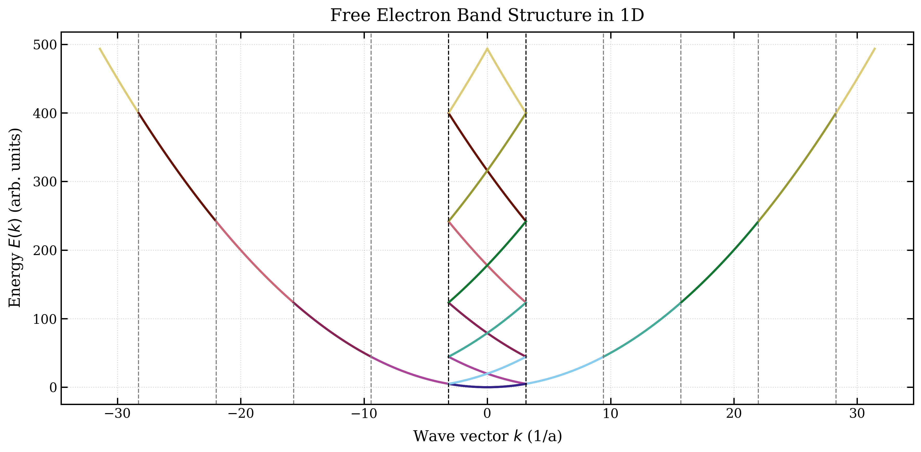
plt.show()Visualization
The following plot shows the free electron band structure with zone folding: