Augmented Plane Wave (APW) Method

Solid State Physics

The Augmented Plane Wave (APW) method is a technique for solving the electronic structure problem in periodic solids. It combines plane waves in the interstitial region with atomic-like radial functions inside muffin-tin spheres around each atom.

Basic Idea

The APW method divides the unit cell into two regions:

Muffin-tin spheres: Around each atom, where the potential is spherically symmetric
Interstitial region: The space between atoms, where plane waves are used

The wavefunction is constructed to be continuous at the muffin-tin boundary, though its derivative may be discontinuous (this limitation is addressed by the LAPW method).

APW Basis Function

The APW basis function is defined piecewise:

ϕ_{k} (r) = ⎩ ⎨ ⎧ l, m \sum C_{l m} u_{l} (r, E) Y_{l}^{m} (\hat{r}), Ω^{- 1/2} e^{i k \cdot r}, ∣ r - R_{α} ∣ < S_{α} ∣ r - R_{α} ∣ \geq S_{α}

where:

$u_{l} (r, E)$ is the radial solution of the Schrödinger equation at energy $E$
$Y_{l}^{m}$ are spherical harmonics
$S_{α}$ is the muffin-tin radius
$Ω$ is the unit cell volume

Boundary Matching

Using the Rayleigh expansion of plane waves:

e^{i k \cdot r} = 4 π ℓ = 0 \sum \infty m = - ℓ \sum ℓ i^{ℓ} j_{ℓ} (k r) Y_{ℓ}^{m *} (\hat{k}) Y_{ℓ}^{m} (\hat{r})

the coefficients are determined by matching at the muffin-tin boundary:

C_{l m} = Ω^{- 1/2} 4 π i^{l} Y_{l}^{m *} (\hat{k}) \frac{j _{l} ( k r _{MT} )}{u _{l} ( r _{MT} , E )}

where $j_{l}$ are spherical Bessel functions and $r_{MT}$ is the muffin-tin radius.

Radial Schrödinger Equation

Inside the muffin-tin, the radial wavefunction $u_{l} (r)$ satisfies:

- \frac{1}{r} \frac{d ^{2}}{d r ^{2}} (r u_{l}) + \frac{l ( l + 1 )}{r ^{2}} u_{l} + V (r) u_{l} = E u_{l}

This is solved using the Numerov method for numerical integration.

Python Implementation

The following code implements the APW method and plots the wavefunction:

import scipy
import numpy as np
import matplotlib.pyplot as plt
import matplotlib as mpl
from scipy.special import spherical_jn

def set_publication_style():
    """Set publication-quality matplotlib style."""
    mpl.rcParams.update({
        'font.family': 'serif',
        'font.size': 12,
        'axes.labelsize': 14,
        'axes.titlesize': 16,
        'axes.linewidth': 1.2,
        'axes.labelpad': 8,
        'axes.titlepad': 10,
        'xtick.labelsize': 12,
        'ytick.labelsize': 12,
        'xtick.direction': 'in',
        'ytick.direction': 'in',
        'xtick.top': True,
        'ytick.right': True,
        'xtick.major.size': 6,
        'ytick.major.size': 6,
        'xtick.major.width': 1.2,
        'ytick.major.width': 1.2,
        'legend.fontsize': 12,
        'legend.frameon': False,
        'lines.linewidth': 2,
        'lines.markersize': 6,
        'figure.dpi': 100,
        'savefig.dpi': 300,
        'savefig.bbox': 'tight'
    })

set_publication_style()

def Numerov(F, dx, f0=0.0, f1=1e-3):
    """
    Numerov method for solving second-order ODEs.
    
    Solves: d^2y/dx^2 = F(x) * y(x)
    """
    Nmax = len(F)
    dx = float(dx)
    Solution = np.zeros(Nmax, dtype=float)
    Solution[0] = f0
    Solution[1] = f1
    h2 = dx * dx
    h12 = h2 / 12
    
    w0 = (1 - h12 * F[0]) * Solution[0]
    Fx = F[1]
    w1 = (1 - h12 * Fx) * Solution[1]
    Phi = Solution[1]
    
    for i in range(2, Nmax):
        w2 = 2 * w1 - w0 + h2 * Phi * Fx
        w0 = w1
        w1 = w2
        Fx = F[i]
        Phi = w2 / (1 - h12 * Fx)
        Solution[i] = Phi
    
    return Solution

def startSol(Z, l, r):
    """
    Starting solution for Numerov algorithm.
    Derived from asymptotic expansion at zero.
    """
    return r**(l+1) * (1 - Z*r/(l+1))

def CRHS(E, l, R, Veff):
    """
    Compute right-hand side for radial Schrödinger equation.
    
    Parameters:
        E: Energy
        l: Angular momentum quantum number
        R: Radial coordinate array
        Veff: Effective potential array
    
    Returns:
        RHS array for Numerov method
    """
    N = len(R)
    RHS = np.zeros(N, dtype=float)
    
    for i in range(N):
        # Radial Schrödinger: -1/r * d^2/dr^2 * r + l(l+1)/r^2 + V
        # Rearranged: d^2u/dr^2 = [2(-E + l(l+1)/(2r^2) + V)] * u
        RHS[i] = 2 * (-E + 0.5 * l * (l + 1) / (R[i] * R[i]) + Veff[i])
    
    return RHS

def extrapolate(x, x0, x1, f0, f1):
    """Linear extrapolation."""
    return f0 + (f1 - f0) * (x - x0) / (x1 - x0)

def ashcroft_potential_array(r, Z=1, rc=0.89, r1=0.4, e2=14.4):
    """
    Ashcroft empty-core pseudopotential.
    
    Parameters:
        r: Radial distance array
        Z: Valence charge
        rc: Core radius
        r1: Inner radius (flat region)
        e2: e^2 / (4πε₀) in eV·Å
    """
    A = -Z * e2 / rc
    B = Z * e2 / rc**2
    x2 = rc - r1
    
    # Cubic interpolation coefficients
    M = np.array([[x2**3, x2**2], [3*x2**2, 2*x2]])
    a, b = np.linalg.solve(M, np.array([A, B]))
    
    V = np.zeros_like(r)
    for i, ri in enumerate(r):
        if ri <= r1:
            V[i] = 0.0
        elif ri < rc:
            x = ri - r1
            V[i] = a * x**3 + b * x**2
        else:
            V[i] = -Z * e2 / ri
    
    return V

# Parameters
rmt = 3.0  # Muffin-tin radius (Å)
vol = 1.0  # Unit cell volume
Z = 1      # Atomic number
l = 0      # Angular momentum (s-wave)
E = 1.0    # Energy parameter

# Radial grid
R0 = np.linspace(0, rmt, 1000, endpoint=True)
R0[0] = 1e-5  # Avoid division by zero
Veff = ashcroft_potential_array(R0, Z=Z)

# Solve radial Schrödinger equation
crhs = CRHS(E, l, R0, Veff)
crhs[0] = 0  # Boundary condition at origin
ur = Numerov(crhs, (R0[-1] - R0[0]) / (len(R0) - 1.0))

# Normalize: ∫ r^2 u_l^2 dr = 1
norm = np.sqrt(scipy.integrate.simpson(ur * ur, x=R0))
ur /= norm

# Convert to wavefunction: ψ = u/r
psi = ur / R0
psi[0] = extrapolate(R0[0], R0[1], R0[2], ur[1]/R0[1], ur[2]/R0[2])

# Construct APW wavefunction
q = 3.0  # Wave vector magnitude
Y_00 = 0.5 * np.sqrt(1 / np.pi)  # Spherical harmonic Y_0^0

def apw_radial_s():
    """
    APW radial wavefunction inside muffin-tin.
    Matches plane wave at boundary.
    """
    # Coefficient: 4π * j_l(k*r_MT) / u_l(r_MT) * Y_00^2
    return 4 * np.pi * spherical_jn(0, q * rmt) / psi[-1] * psi * Y_00**2

# Plot results
fig, axes = plt.subplots(1, 2, figsize=(14, 5))

# Left: Potential
axes[0].plot(R0, Veff, 'b-', linewidth=2)
axes[0].axvline(rmt, color='r', linestyle='--', linewidth=2, label='Muffin-tin radius')
axes[0].set_xlabel('r (Å)')
axes[0].set_ylabel('V(r) (eV)')
axes[0].set_title('Ashcroft Pseudopotential')
axes[0].legend()
axes[0].grid(True, alpha=0.3)

# Right: APW wavefunction
# Inside muffin-tin
apw_inside = apw_radial_s()
axes[1].plot(R0, apw_inside, 'b-', linewidth=2, label='APW (inside MT)')

# Outside muffin-tin (plane wave)
inter = np.linspace(rmt, 2*rmt, 100)
apw_outside = 4 * np.pi * spherical_jn(0, inter * q) * Y_00**2
axes[1].plot(inter, apw_outside, 'r-', linewidth=2, label='Plane wave (outside)')

axes[1].axvline(rmt, color='k', linestyle='--', linewidth=1, alpha=0.5)
axes[1].set_xlabel('Distance (Å)')
axes[1].set_ylabel('Wavefunction')
axes[1].set_title('Augmented Plane Wave')
axes[1].legend()
axes[1].grid(True, alpha=0.3)

plt.tight_layout()
plt.savefig('figures/apw_wavefunction.png', dpi=300, bbox_inches='tight')
plt.show()

# Verify continuity at boundary
print(f"Wavefunction at boundary (inside): {apw_inside[-1]:.6f}")
print(f"Wavefunction at boundary (outside): {apw_outside[0]:.6f}")
print(f"Continuity error: {abs(apw_inside[-1] - apw_outside[0]):.2e}")

Visualization

The following plot shows the APW wavefunction, with the radial solution inside the muffin-tin sphere and the plane wave outside:

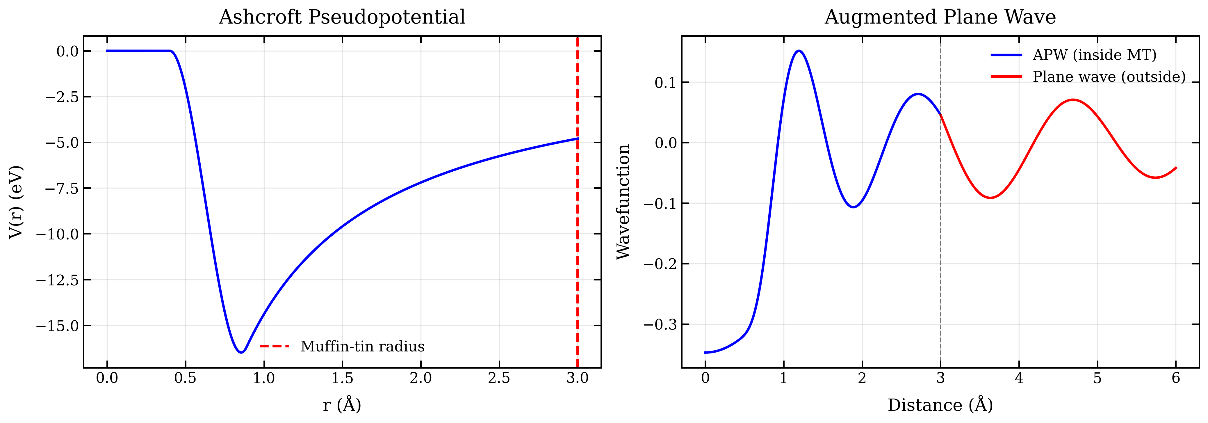
Key Features

Piecewise basis function: radial inside muffin-tin, plane wave outside
Radial solution computed using Numerov method
Boundary matching using Rayleigh expansion
Continuous wavefunction at muffin-tin boundary
Discontinuous derivative (limitation addressed by LAPW)

Limitations

The APW method has a key limitation:

Discontinuous derivative: The derivative of the wavefunction is not continuous at the muffin-tin boundary
Energy-dependent basis: The radial functions depend on energy, making the eigenvalue problem nonlinear

These limitations led to the development of the Linearized APW (LAPW) method, which uses energy derivatives to linearize the problem and ensure continuous derivatives.

Historical Context

The APW method was developed by J.C. Slater in 1937 and was one of the first methods to give quantitative results for periodic solids. It predates both DFT and pseudopotentials, demonstrating the power of the independent particle approximation.

Applications

The APW method and its linearized version (LAPW) are used for:

Band structure calculations
Electronic structure of transition metals
Magnetic materials
Strongly correlated systems
All-electron calculations (no pseudopotential needed)