LAPW Method

Solid State Physics

The Linearized Augmented Plane Wave (LAPW) method is a powerful technique for solving the electronic structure problem in periodic solids. It combines plane waves in the interstitial region with atomic-like functions inside muffin-tin spheres.

Basic Idea

The LAPW method divides the unit cell into two regions:

Muffin-tin spheres: Around each atom, where the potential is nearly spherically symmetric
Interstitial region: The space between atoms, where the potential is relatively smooth

Different basis functions are used in each region and matched at the boundaries.

LAPW Basis Functions

The LAPW basis function is defined piecewise:

ϕ_{k_{n}} (r) = ⎩ ⎨ ⎧ l, m \sum [a_{l m} u_{l} (E_{l}, r) + b_{l m} \overset{u}{˙}_{l} (E_{l}, r)] Y_{l}^{m} (\hat{r}), Ω^{- 1/2} e^{i k_{n} \cdot r}, ∣ r - R_{α} ∣ < S_{α} ∣ r - R_{α} ∣ \geq S_{α}

where:

$u_{l} (E_{l}, r)$ is the radial solution of the Schrödinger equation at energy $E_{l}$
$\overset{u}{˙}_{l} (E_{l}, r)$ is the energy derivative of the radial solution
$Y_{l}^{m}$ are spherical harmonics
$k_{n} = k + K_{n}$ where $K_{n}$ are reciprocal lattice vectors
$S_{α}$ is the muffin-tin radius for atom $α$

Radial Schrödinger Equation

Inside the muffin-tin sphere, the radial wavefunction $u_{l} (r)$ satisfies:

h_{l} u_{l} - E_{l} u_{l} = 0

where the radial Hamiltonian is:

h_{l} = - \frac{1}{r} \frac{d ^{2}}{d r ^{2}} r + \frac{l ( l + 1 )}{r ^{2}} + V (r)

The energy derivative $\overset{u}{˙}_{l}$ satisfies:

h_{l} \overset{u}{˙}_{l} - E_{l} \overset{u}{˙}_{l} = u_{l}

This is solved using the Numerov method for numerical integration.

Boundary Matching

The coefficients $a_{l m}$ and $b_{l m}$ are determined by matching the basis function and its derivative at the muffin-tin boundary. Using the Rayleigh expansion of plane waves:

e^{i k \cdot r} = 4 π ℓ = 0 \sum \infty m = - ℓ \sum ℓ i^{ℓ} j_{ℓ} (k r) Y_{ℓ}^{m} (\hat{r}) Y_{ℓ}^{m *} (\hat{k})

the matching conditions give:

a_{l} = j_{l}^{'} (k R) \overset{u}{˙}_{l} (R) - j_{l} (k R) \overset{u}{˙}_{l}^{'} (R)

b_{l} = j_{l} (k R) u_{l}^{'} (R) - j_{l}^{'} (k R) u_{l} (R)

where $R$ is the muffin-tin radius and $j_{l}$ are spherical Bessel functions.

Generalized Eigenvalue Problem

The electronic structure problem becomes a generalized eigenvalue problem:

H c = ES c

where:

$H_{nm} = ⟨ ϕ_{k_{n}} ∣ H ∣ ϕ_{k_{m}} ⟩$ is the Hamiltonian matrix
$S_{nm} = ⟨ ϕ_{k_{n}} ∣ ϕ_{k_{m}} ⟩$ is the overlap matrix
$c$ are the expansion coefficients

The overlap matrix is not the identity because the basis functions are not orthogonal (unlike pure plane waves).

Python Implementation

A simplified LAPW implementation using Numerov for the radial part:

import numpy as np
import scipy
from scipy.special import spherical_jn
import matplotlib.pyplot as plt
import matplotlib as mpl

def set_publication_style():
    """Set publication-quality matplotlib style."""
    mpl.rcParams.update({
        'font.family': 'serif',
        'font.size': 12,
        'axes.labelsize': 14,
        'axes.titlesize': 16,
        'axes.linewidth': 1.2,
        'axes.labelpad': 8,
        'axes.titlepad': 10,
        'xtick.labelsize': 12,
        'ytick.labelsize': 12,
        'xtick.direction': 'in',
        'ytick.direction': 'in',
        'xtick.top': True,
        'ytick.right': True,
        'xtick.major.size': 6,
        'ytick.major.size': 6,
        'xtick.major.width': 1.2,
        'ytick.major.width': 1.2,
        'legend.fontsize': 12,
        'legend.frameon': False,
        'lines.linewidth': 2,
        'lines.markersize': 6,
        'figure.dpi': 100,
        'savefig.dpi': 300,
        'savefig.bbox': 'tight'
    })

set_publication_style()

def Numerov(F, dx, f0=0.0, f1=1e-3):
    """
    Numerov method for solving second-order ODEs.
    
    Solves: d^2y/dx^2 = F(x) * y(x)
    """
    Nmax = len(F)
    dx = float(dx)
    Solution = np.zeros(Nmax, dtype=float)
    Solution[0] = f0
    Solution[1] = f1
    h2 = dx * dx
    h12 = h2 / 12
    
    w0 = (1 - h12 * F[0]) * Solution[0]
    Fx = F[1]
    w1 = (1 - h12 * Fx) * Solution[1]
    Phi = Solution[1]
    
    for i in range(2, Nmax):
        w2 = 2 * w1 - w0 + h2 * Phi * Fx
        w0 = w1
        w1 = w2
        Fx = F[i]
        Phi = w2 / (1 - h12 * Fx)
        Solution[i] = Phi
    
    return Solution

def NumerovGen(F, U, dx, f0=0.0, f1=1e-3):
    """
    Generalized Numerov method for inhomogeneous ODEs.
    
    Solves: d^2y/dx^2 = F(x) * y(x) + U(x)
    """
    Nmax = len(F)
    dx = float(dx)
    Solution = np.zeros(Nmax, dtype=float)
    Solution[0] = f0
    Solution[1] = f1
    
    h2 = dx * dx
    h12 = h2 / 12
    
    w0 = Solution[0] * (1 - h12 * F[0]) - h12 * U[0]
    w1 = Solution[1] * (1 - h12 * F[1]) - h12 * U[1]
    Phi = Solution[1]
    
    for i in range(2, Nmax):
        Fx = F[i]
        Ux = U[i]
        w2 = 2 * w1 - w0 + h2 * (Phi * Fx + Ux)
        w0 = w1
        w1 = w2
        Phi = (w2 + h12 * Ux) / (1 - h12 * Fx)
        Solution[i] = Phi
    
    return Solution

def CRHS(E, l, R, Veff):
    """
    Compute right-hand side for radial Schrödinger equation.
    
    Parameters:
        E: Energy
        l: Angular momentum quantum number
        R: Radial coordinate array
        Veff: Effective potential array
    
    Returns:
        RHS array for Numerov method
    """
    N = len(R)
    RHS = np.zeros(N, dtype=float)
    
    for i in range(N):
        # Radial Schrödinger equation: -1/r * d^2/dr^2 * r + l(l+1)/r^2 + V
        # Rearranged for Numerov: d^2u/dr^2 = [2(-E + l(l+1)/(2r^2) + V)] * u
        RHS[i] = 2 * (-E + 0.5 * l * (l + 1) / (R[i] * R[i]) + Veff[i])
    
    return RHS

def ashcroft_potential(r, Z=1, rc=0.89, r1=0.4, e2=14.4):
    """
    Ashcroft empty-core pseudopotential.
    
    Parameters:
        r: Radial distance array
        Z: Valence charge
        rc: Core radius
        r1: Inner radius (flat region)
        e2: e^2 / (4πε₀) in eV·Å
    """
    A = -Z * e2 / rc
    B = Z * e2 / rc**2
    x2 = rc - r1
    
    # Cubic interpolation coefficients
    M = np.array([[x2**3, x2**2], [3*x2**2, 2*x2]])
    a, b = np.linalg.solve(M, np.array([A, B]))
    
    V = np.zeros_like(r)
    for i, ri in enumerate(r):
        if ri <= r1:
            V[i] = 0.0
        elif ri < rc:
            x = ri - r1
            V[i] = a * x**3 + b * x**2
        else:
            V[i] = -Z * e2 / ri
    
    return V

# Example: Solve radial Schrödinger equation for l=0
rmt = 3.0  # Muffin-tin radius
E = 2.0    # Linearization energy
l = 0      # Angular momentum
Z = 1      # Atomic number

# Radial grid
R = np.linspace(1e-5, rmt, 1000, endpoint=True)
Veff = ashcroft_potential(R, Z=Z)

# Solve for u_l
crhs = CRHS(E, l, R, Veff)
crhs[0] = 0.0  # Boundary condition at origin
u_l = Numerov(crhs, (R[-1] - R[0]) / (len(R) - 1.0))

# Normalize: ∫ r^2 u_l^2 dr = 1
norm = np.sqrt(scipy.integrate.simpson(u_l * u_l, x=R))
u_l /= norm

# Solve for energy derivative u_dot
inhom = -2 * u_l
u_dot = NumerovGen(crhs, inhom, (R[-1] - R[0]) / (len(R) - 1.0))

# Orthogonalize u_dot with respect to u_l
alpha = scipy.integrate.simpson(u_l * u_dot, x=R)
u_dot -= alpha * u_l

# Normalize u_dot
norm_dot = np.sqrt(scipy.integrate.simpson(u_dot * u_dot, x=R))
u_dot /= norm_dot

# Plot results
fig, axes = plt.subplots(1, 2, figsize=(12, 5))

# Left: Potential and wavefunctions
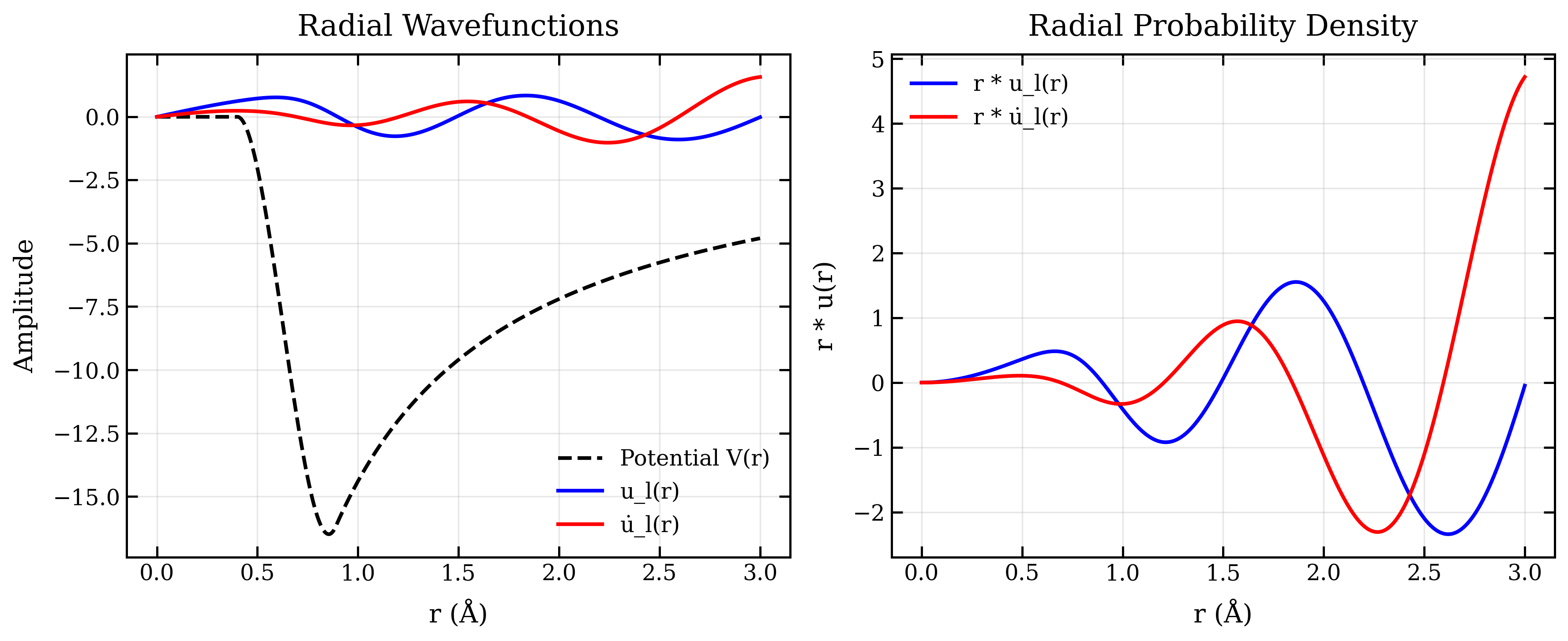
axes[0].plot(R, Veff, 'k--', linewidth=2, label='Potential V(r)')
axes[0].plot(R, u_l, 'b-', linewidth=2, label='u_l(r)')
axes[0].plot(R, u_dot, 'r-', linewidth=2, label='u̇_l(r)')
axes[0].set_xlabel('r (Å)')
axes[0].set_ylabel('Amplitude')
axes[0].set_title('Radial Wavefunctions')
axes[0].legend()
axes[0].grid(True, alpha=0.3)

# Right: Probability density
axes[1].plot(R, R * u_l, 'b-', linewidth=2, label='r * u_l(r)')
axes[1].plot(R, R * u_dot, 'r-', linewidth=2, label='r * u̇_l(r)')
axes[1].set_xlabel('r (Å)')
axes[1].set_ylabel('r * u(r)')
axes[1].set_title('Radial Probability Density')
axes[1].legend()
axes[1].grid(True, alpha=0.3)

plt.tight_layout()
plt.savefig('figures/lapw_radial_wavefunctions.png', dpi=300, bbox_inches='tight')
plt.show()

print(f"Normalization check:")
print(f"  ∫ r^2 u_l^2 dr = {scipy.integrate.simpson(u_l * u_l, x=R):.6f}")
print(f"  ∫ r^2 u_dot^2 dr = {scipy.integrate.simpson(u_dot * u_dot, x=R):.6f}")
print(f"  ∫ r^2 u_l * u_dot dr = {scipy.integrate.simpson(u_l * u_dot, x=R):.6f}")

Visualization

The following plot shows the radial wavefunctions and potential:

Key Features

Piecewise basis functions adapted to the physics of each region
Radial solutions computed using Numerov method
Energy derivatives for linearization
Boundary matching using spherical Bessel functions
Generalized eigenvalue problem with overlap matrix

Advantages

The LAPW method offers several advantages:

Accuracy: Handles both core and valence electrons accurately
Efficiency: Fewer basis functions needed than pure plane waves
Flexibility: Can handle strong potentials near nuclei
All-electron: No pseudopotential approximation needed

Applications

LAPW is widely used in:

Band structure calculations
Density functional theory (DFT) for solids
Magnetic materials
Strongly correlated systems
Transition metal compounds

Historical Context

The LAPW method was developed as an improvement over the Augmented Plane Wave (APW) method. The key innovation is the linearization, which allows the energy to vary while maintaining continuity at the muffin-tin boundary. This was first described by Koelling and Arbman in 1975.