Casida for Paints: Color from Conjugation

A carrot is orange, a tomato is red, and butadiene is colorless — and the same equation explains all three. Color, for a molecule, means absorbing a chunk of the visible spectrum, and a molecule absorbs a photon when it has an electronic excitation at that photon's energy. So "what color is this compound?" is really "where is its lowest bright excitation?", and that is a question time-dependent density functional theory answers directly, through the Casida equations. This page runs real TDDFT on the linear polyene series — conjugated chains of growing length — watches the absorption march from the deep ultraviolet toward the visible as the chain grows, hands the excitation energies to the symbolic-regression engine to extract the law, and tests that law against the real carotenoids — where it captures the mechanism cleanly and misses the absolute wavelength in a way worth understanding.

The excitation is the color

Linear-response TDDFT reduces the question of a molecule's excitations to a single generalized eigenvalue problem, Casida's equation. Its eigenvalues are the excitation energies ${\omega }_I$; its eigenvectors are the transition densities, which set the oscillator strength $f_I$ — how strongly the molecule couples to light at that energy. Solve it, find the lowest root with large $f$, and the absorption wavelength follows immediately:

For a conjugated molecule the bright, low-energy transition is always the same character: an electron promoted from the highest occupied $\pi$ orbital to the lowest unoccupied ${\pi }^{\ast }$ — the HOMO→LUMO $\pi \to {\pi }^{\ast }$ excitation delocalized over the conjugated backbone. Everything about the molecule's color is set by where that one transition sits.

# The bright pi->pi* excitation of a conjugated molecule, from real TDDFT.
# Series: all-trans polyenes CH2=(CH-CH=)_{n-1}CH2, n = 1..6 double bonds.

def tddft_lambda_max(n):
    mol = gto.M(atom=planar_polyene(n), basis='6-31g*', verbose=0)
    mf  = dft.RKS(mol).density_fit(); mf.xc = 'b3lyp'; mf.kernel()   # ground state
    td  = tddft.TDA(mf); td.nstates = 6; td.kernel()                # Casida (TDA)
    f   = td.oscillator_strength()
    e   = td.e * 27.2114                                            # eV
    b   = int(np.argmax(f))            # brightest root = the pi->pi* 1Bu state
    return e[b], 1239.84 / e[b], f[b]  # energy, lambda_max [nm], oscillator strength

A methods trap worth knowing: the triplet instability

There is a real subtlety here, and stepping on it is instructive. Run full TDDFT (the Casida equations with both the excitation and de-excitation blocks) on these polyenes and the shorter chains behave, but from the six-carbon chain onward the calculation returns a spurious excitation at almost zero energy with an enormous oscillator strength — a red flag, not a red dye. The cause is a triplet instability: the closed-shell Kohn–Sham reference for a stretched conjugated system is unstable toward a lower-energy open-shell state, and that instability leaks into the response equations as a near-zero root. The standard cure is the Tamm–Dancoff approximation, which drops the de-excitation coupling block responsible for the instability. TDA systematically blue-shifts the excitation energies by a few tenths of an eV, but it is stable, and for polyenes it is the appropriate tool. Knowing when your method is lying to you — and why — is the difference between running a black box and using it.

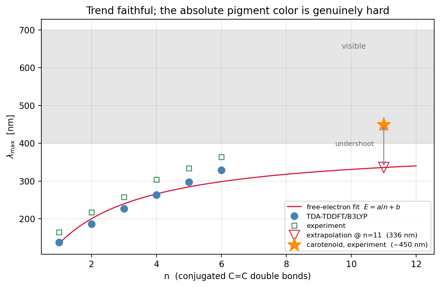
The red-shift, computed

Across the series the bright $\pi \to {\pi }^{\ast }$ absorption red-shifts steadily as the conjugated chain lengthens — the central result, and it reproduces the experimental trend faithfully:

TDA-TDDFT / B3LYP / 6-31G*  on all-trans polyenes  (n = C=C double bonds)

  n=1   C2H4     E=8.98 eV    lambda_max=138 nm    exp=165 nm    (-27)
  n=2   C4H6     E=6.65 eV    lambda_max=186 nm    exp=217 nm    (-31)
  n=3   C6H8     E=5.46 eV    lambda_max=227 nm    exp=258 nm    (-31)
  n=4   C8H10    E=4.71 eV    lambda_max=263 nm    exp=304 nm    (-41)
  n=5   C10H12   E=4.17 eV    lambda_max=297 nm    exp=334 nm    (-37)
  n=6   C12H14   E=3.77 eV    lambda_max=329 nm    exp=364 nm    (-35)

  MAE vs experiment = 33 nm        trend correlation  r = 0.9991

  law E(n):  symbolic regression prefers   E ~ -2.91 log(n) + 8.82   (RMSE 0.13 eV)
             free-electron form            E =  6.09/n   + 3.14      (RMSE 0.30 eV)
             -> log fits better in-range but -> -inf; only a/n+b has a finite gap

  extrapolate to carotenoids (n~11):  336 nm   vs   experiment ~450 nm   (undershoot)

Every point sits about 30 nm short of experiment — a mean absolute error of 33 nm, and, more tellingly, a trend correlation of $r=0.9991$. That near-constant offset is TDA/B3LYP's systematic blue-shift: the method overestimates the $\pi \to {\pi }^{\ast }$ energy by a few tenths of an eV, uniformly, sliding every wavelength toward the ultraviolet while preserving the shape of the trend almost perfectly. Color is about where the absorption moves as the molecule changes, and that motion is reproduced to better than a percent.

The mechanism is the particle in a box. The $\pi$ electrons are delocalized along the conjugated backbone like a free electron confined to a wire; lengthening the chain lengthens the box, the quantized levels $E_k\propto k^2/L^2$ squeeze together, and the HOMO→LUMO gap — the absorption energy — shrinks. More conjugation, smaller gap, redder color. The free-electron model even suggests the functional form, $E\propto 1/n$ — though the fit has a twist worth savoring.

Hand the six excitation energies to the symbolic-regression engine and its best simple law is not the free-electron $1/n$ but a logarithm, $E\approx -2.9\ln n+8.8$, which fits the points more than twice as tightly (RMSE 0.13 vs 0.30 eV). Over $n=1\text{–}6$ the logarithm genuinely is the better description — and it is physically wrong: $\ln n\to \infty$ means the gap collapsing without bound, an infinite chain absorbing at infinite wavelength. The free-electron form $E=a/n+b$ fits worse in-range but has the one feature the physics demands — a finite intercept $b$, the gap of the infinite chain. This is the symbolic-regression page's warning arriving on real data: the tightest fit inside your data is not the law that extrapolates. Choosing between two equally-good-in-range fits is where physics, not the fitter, has to speak — here through the demand that an infinite conjugated wire still have a finite gap.

From spectrum to swatch

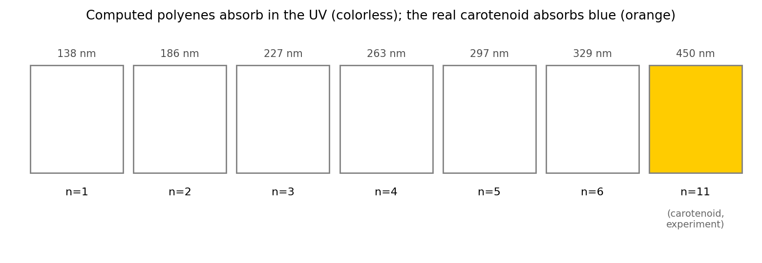
A pigment's perceived color is, to a first approximation, the complement of what it absorbs: absorb blue light and the reflected remainder looks orange; absorb nothing in the visible and the compound is colorless. That is why the short polyenes are clear liquids — their absorption is buried in the ultraviolet — and it is why the extrapolated carotenoid, with its absorption pushed into the blue, comes out orange. The swatch on the right is not a photograph; it is the computed absorption wavelength run through a wavelength-to-color map and complemented. The physics that colors it is the same physics that colors a carrot.

So does the law predict the orange of a carrot? Not quite — and the way it misses is the point. Extrapolate the free-electron fit to the eleven double bonds of $\beta$-carotene and it lands at 336 nm, still in the near-ultraviolet, more than 100 nm short of the real $\sim 450$ nm that makes carotenoids orange. Three things conspire: TDA's systematic blue-shift, an asymptotic gap the short chains cannot pin down (the fit's 3.1 eV intercept against polyacetylene's true $\sim 1.8$ eV), and the multireference character of long polyenes that strains any single-reference method — the same instability that forced TDA in the first place. The mechanism is unambiguous and the trend is quantitative; the absolute color of a real pigment, extrapolated across a factor of two in chain length, is genuinely hard. That gap between a clean trend and a stubborn absolute number is what computational pigment design actually looks like.

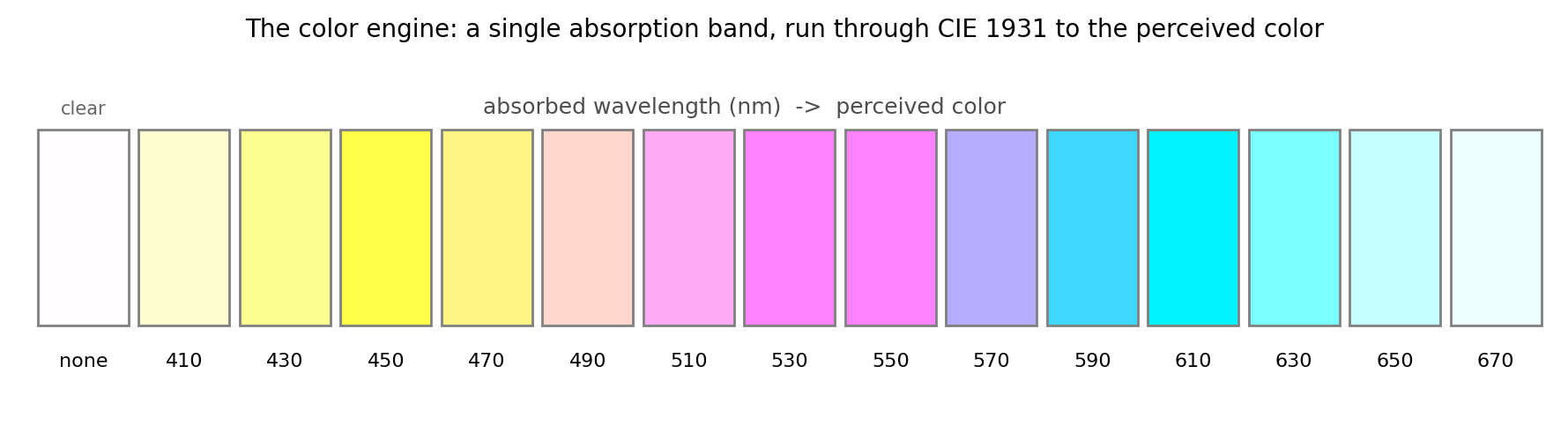
Beyond λ_max: the real color engine

The complement rule is a cartoon — a good one, but a cartoon. A real pigment's color is not set by a single wavelength; it is set by the whole absorption band, seen through the eye. Turning a computed spectrum into an actual color is a deterministic pipeline: broaden the TDDFT excitations into an absorption curve, attenuate daylight through it by Beer–Lambert, and convolve what is left with the CIE 1931 color-matching functions — the tabulated response of the three cone types — to land in the sRGB a screen can display. Sweep a single synthetic absorption band across the visible and the complements fall out exactly:

This is the piece the swatch above only gestured at, and it works for any molecule, not just polyenes. Which sharpens where the difficulty actually is, because predicting a molecule's color factors cleanly in two:

The first factor is the pipeline above — deterministic, validated, done. The second is where the difficulty lives, and cheap TDDFT is not yet good enough to carry it for an arbitrary dye. Screen a handful of small molecules and the pattern is stark: the colorless controls come out right — naphthalene and anthracene absorb only in the ultraviolet, so the engine returns white — but indigo, a deep blue whose absorption sits at 605 nm, comes back from B3LYP with its lowest band near 400 nm, predicting yellow. A one-electron-volt error in the excitation energy flips the hue to its opposite. Optimizing the geometry and adding an implicit solvent each nudge the number the right way, but neither closes a gap that large.

So the shape of computational pigment design is this: the colorimetry is easy and the quantum chemistry is hard. The color engine (scripts/gen_dye_color.py) is a solved, reusable tool; the bottleneck — the thing worth methodological effort — is getting an excitation energy right to a tenth of an electron-volt for a molecule no one has yet measured. That is where the field's method development lives, and it is why a screening pipeline that generates candidate colorants is only ever as good as the excited-state method underneath it.

What this does and doesn't get right

• The trend is robust; the absolute numbers are approximate. TDA/B3LYP blue-shifts the polyene $\pi \to {\pi }^{\ast }$ energies systematically, so every computed ${\lambda }_{\max }$ sits short of experiment by a roughly constant offset. The red-shift with chain length — the thing that sets color — is reproduced faithfully.
• Real pigments are not gas-phase polyenes. Solvent shifts, vibronic structure (the absorption is a band, not a line), aggregation, and the substituents of an actual dye all move the number. A quantitative color needs the full spectrum convolved with the eye's response, not a single ${\lambda }_{\max }$.
• Long conjugation is where TDDFT strains. The same triplet instability that forced TDA is a symptom of the multireference character that grows with chain length; for the true carotenoids a single-reference method is being pushed near its limit, which is why we extrapolate a law from the tractable short chains rather than compute $\beta$-carotene directly.

Reproduce it

scripts/gen_casida_paints.py builds the planar all-trans polyenes from scratch (bond-alternating geometry, no conformer lottery), runs B3LYP + TDA in PySCF, and extracts the bright $\pi \to {\pi }^{\ast }$ state for $n=1$ to $6$. It then imports the genetic-programming engine from the symbolic-regression page — the same code that rediscovered Kepler's law — to recover $E(n)$ from the computed points, and maps each ${\lambda }_{\max }$ to a color swatch. Change the functional, the basis, or the series and watch the trend hold and the offset move.