When a Linear Model Stops Being Linear

Linear regression's superpower is interpretability. Each coefficient says how much one input contributes to the output — read it, regulate by it, write a paper about it. But that superpower only holds when the model is small. As soon as the data is complicated enough to need a big basis — polynomial degree 25, 300 radial basis functions, 175 random Fourier features — the model is technically still "linear in its parameters", but the parameters themselves are a wall of plus-and-minus hundreds with no story to tell. The model class is the same. The interpretability is gone.

Once that's true, the linear basis has nothing left over the alternative: an MLP at the same parameter budget. Or does it? This page runs two rigorous head-to-head experiments — 10 random seeds, cross-validated regularization on every method, matched parameter counts — and the answer turns out to be more nuanced than the slogan suggests. When the basis matches the data, the linear method wins. When it doesn't, the MLP wins. What the linear method gives up is the freedom to ever be wrong about that match.

The protocol

Every method gets the same fair treatment so the comparison can't be gamed by hand-picked hyperparameters:

For each of 10 random seeds (each producing a different ground-truth target
and a different draw of training samples) every method gets the same fair
treatment:

  1. Split: 500 noisy training points, 100 noisy validation points,
     a separate noise-free test set against the actual truth.
  2. Cross-validate: for each linear basis, choose the ridge lambda
     from {1e-8, 1e-6, 1e-4, 1e-2, 1}. For the MLP, choose weight decay
     from {0, 1e-5, 1e-4, 1e-3} using early stopping on validation MSE.
  3. Refit on train + val using the best hyperparameter.
  4. Evaluate on the noise-free test set.

Each method's parameter count is held within +/- 15% so the comparison
is at matched model capacity (not at matched depth of pocket).

Experiment 1: 2D Gaussian bumps

The truth is a sum of seven Gaussian bumps on the unit square, random centers and amplitudes, all with width $\sigma =0.10$:

Four methods, all at roughly 340 parameters: polynomial regression (total degree 25, 351 features), RBF regression (300 random centers, ${\sigma }_{\text{RBF}}=0.08$), random Fourier features (175 frequencies → 350 cos+sin columns), and an MLP with 2 hidden layers of 16 tanh units (337 trainable parameters).

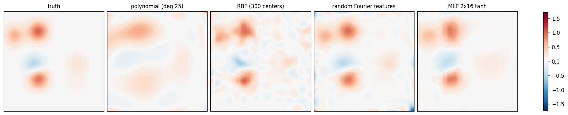
Eyeball test on a single seed (above): the polynomial rings, RBF is clean, Fourier is clean with some background texture, MLP is clean but slightly softer than RBF. The aggregated numbers across 10 seeds:

=== 2D Gaussian bumps, 10 seeds ===
method                    params      train MSE (mean +/- sd)    test MSE (mean +/- sd)
----------------------------------------------------------------------------------------------
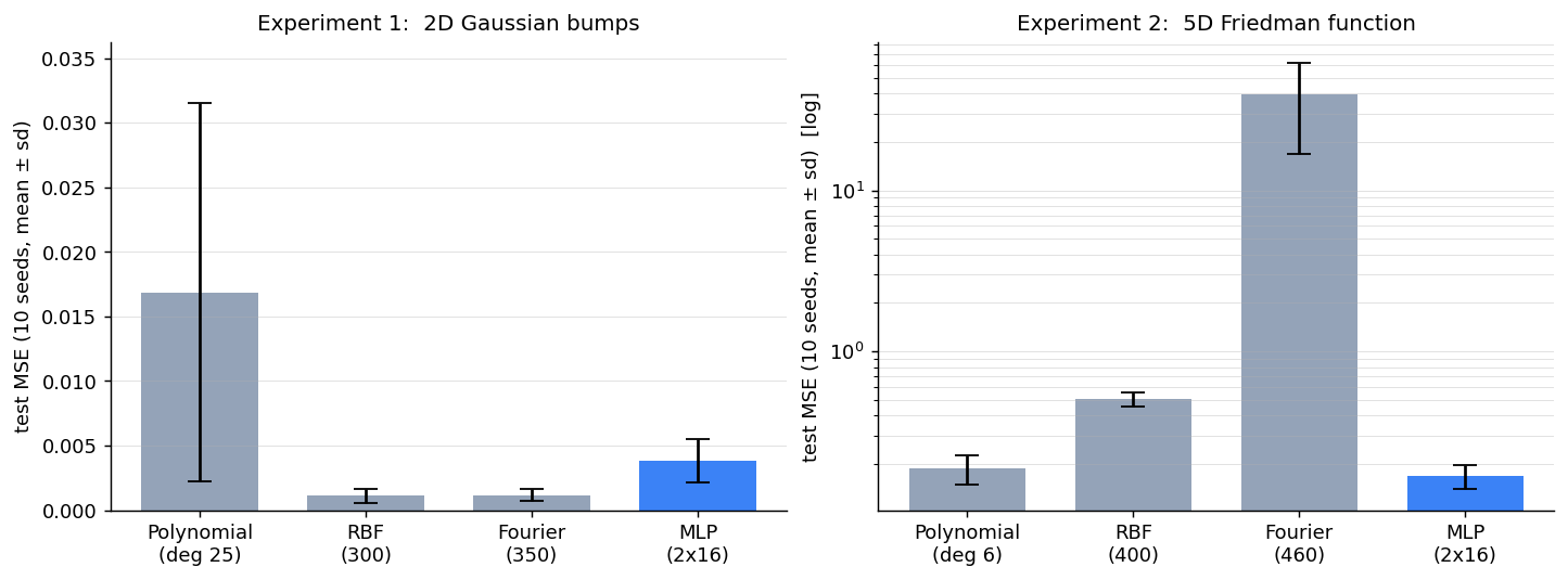
Polynomial (deg 25)          351      0.00735 +/- 0.00328         0.01688 +/- 0.01465
RBF (300 centers)            300      0.00217 +/- 0.00050         0.00110 +/- 0.00056
Random Fourier features      350      0.00208 +/- 0.00019         0.00117 +/- 0.00049
MLP 2x16 tanh                337      0.00505 +/- 0.00137         0.00384 +/- 0.00168

paired wins on test MSE, MLP vs other (out of 10):
  MLP < Polynomial             10/10
  MLP < RBF                     0/10
  MLP < Random Fourier feats    1/10

coefficient magnitudes for linear bases (averaged over seeds):
  Polynomial    mean max|w| = 682.0    mean ||w||2 = 3174.1
  RBF           mean max|w| =   0.5    mean ||w||2 =    1.6
  Fourier feats mean max|w| =   0.1    mean ||w||2 =    0.4

RBF wins. Not the MLP — RBF. 10 out of 10 seeds, by a factor of ~3.5 in test MSE. And the reason isn't subtle: the truth is a sum of Gaussians, and RBF features are Gaussians. The basis matches the data exactly. Random Fourier features are almost as good (also a kernel approximation, similar in spirit). Polynomial does the worst because total-degree polynomials suffer from Runge-style ringing at the boundary, and seven sharp bumps create exactly the kind of localized structure polynomials handle badly. The MLP comes in third — competent, but it has to spend its 337 parameters learning what RBFs got for free as a hard-coded prior.

This is the strongest possible case for a linear basis. The data matched the basis perfectly; nothing the MLP can do will recover the statistical efficiency the basis gives you when the prior is right. The lesson of Experiment 1 is the part of the argument that often gets skipped: when you can name the basis your data lives in, the linear method is hard to beat.

Experiment 2: Friedman 5D

Now break the basis match. The Friedman (1991) regression benchmark mixes a sinusoidal interaction, a quadratic, and two linear terms in five input dimensions:

with $x\in [0,1{]}^5$ and noise $\epsilon \sim \mathcal{N}(0,1)$. None of the three classical bases is obviously well-matched: the sinusoid wants Fourier features, the quadratic wants polynomials, the linear terms want… linear features. Each basis is right about part of the function and wrong about the rest.

The polynomial basis also starts to bite back. In 2D, total degree 25 cost 351 features; in 5D, total degree 25 would cost $\left(\genfrac{}{}{0ex}{}{30}{5}\right)=142,506$ features. We drop to degree 6 ($\left(\genfrac{}{}{0ex}{}{11}{5}\right)=462$ features) to stay in the parameter budget. The MLP, importantly, doesn't change architecture between experiments — it's still 2 hidden layers of 16 tanh units, now with a 5-dimensional input, totaling 385 parameters.

=== Friedman 5D, 10 seeds ===
method                    params      train MSE (mean +/- sd)    test MSE (mean +/- sd)
----------------------------------------------------------------------------------------------
Polynomial (deg 6)           462      0.8631 +/- 0.1374           0.1876 +/- 0.0388
RBF (400 centers)            400      0.9020 +/- 0.1460           0.5067 +/- 0.0503
Random Fourier features      460     10.1913 +/- 6.3850          39.2044 +/- 22.2737
MLP 2x16 tanh                385      0.9718 +/- 0.0279           0.1689 +/- 0.0286

paired wins on test MSE, MLP vs other (out of 10):
  MLP < Polynomial              7/10
  MLP < RBF                    10/10
  MLP < Random Fourier feats   10/10

coefficient magnitudes for linear bases (averaged over seeds):
  Polynomial    mean max|w| =  27.1    mean ||w||2 =   62.7
  RBF           mean max|w| =  59.6    mean ||w||2 =  350.5
  Fourier feats mean max|w| =  17.1    mean ||w||2 =   28.6

The MLP wins. 7/10 paired comparisons against the polynomial (the closest competitor) and 10/10 against everything else. The polynomial isn't actually bad — Friedman has explicit algebraic structure that low-degree polynomials catch — but the MLP edges it out using fewer parameters. RBF and Fourier features fall apart for opposite reasons. RBFs are isotropic local features in 5D, where "local" requires exponentially many centers to cover the space, and 400 random centers do a poor job. Random Fourier features at frequency scale $2\pi$ are even worse: in 5D, random frequencies aim mostly in directions Friedman doesn't care about, so the basis spends almost all its capacity reconstructing high-frequency noise that isn't there. Test MSE of $39$ ± $22$ is a complete failure.

This is the case the original argument was about. When the data doesn't match any single classical basis, the MLP wins because it doesn't have to commit to a basis.

The interpretability check

Even on the experiment where the linear basis wins, none of the methods is interpretable. The RBF that wins Experiment 1 has 300 coefficients, mean ${\ell }_2$ norm 1.6 — small in absolute terms, but still 300 numbers summing into one function value. The Fourier basis is similar. The polynomial is comically un-interpretable: 351 coefficients with average max $|w|$ of 682, summing into a function value that ought to live in $[-1,+1]$. Reading the polynomial coefficients is reading the surface tension of a soap bubble.

"Linear in the parameters" is a mathematical property of how you fit the model, not a property of how a human reads the fit. The linear regression with two coefficients (slope and intercept) is interpretable because two numbers are interpretable. The linear regression with 351 coefficients is not interpretable in any sense a human cares about — even if it wins on accuracy.

The kernel-methods view

There's a clean theoretical reason for everything above, and it's worth stating because it removes the magic. Every linear basis defines a kernel via $K(x,x^{\prime })=\varphi (x{)}^{\top }\varphi (x^{\prime })$, and the linear regression in that basis is equivalent to kernel ridge regression in a reproducing-kernel Hilbert space (RKHS). So:

• Polynomial features give the polynomial kernel $K(x,x^{\prime })=(1+x^{\top }{x}^{\prime }{)}^d$.
• RBF features give an approximation to the Gaussian kernel $K(x,x^{\prime })=\exp (-\Vert x-x^{\prime }{\Vert }^2/2{\sigma }^2)$.
• Random Fourier features (Rahimi & Recht, 2007) are a Monte Carlo approximation to a shift-invariant kernel $K(x,x^{\prime })=\int p(\omega )e^{i\omega \cdot (x-x^{\prime })}d\omega$.

Picking a linear basis is therefore picking a kernel — picking, in effect, what "smoothness" or "similarity" means for your problem. When the chosen kernel matches the truth, you get statistical efficiency that the MLP can't match at the same parameter count.

And the MLP? At infinite width, an MLP trained with gradient descent is itself a kernel method, with the kernel given by the neural tangent kernel (Jacot, Gabriel, & Hongler, 2018). What the MLP buys you is a kernel whose shape adapts during training — at finite width and away from the lazy regime, the network's effective kernel co-evolves with the data, picking up features the loss surface rewards. That's the freedom the linear method doesn't have. It's also why, on Friedman 5D where no fixed kernel matches well, the MLP wins.

What this whole argument actually says

If you can name the basis your data lives in — true Fourier modes, sums of Gaussians, low-degree polynomials, splines on a known grid — use a linear method. You get closed-form inference, calibrated uncertainty via marginal likelihood, fast hyperparameter tuning, and statistical efficiency the MLP can't match. The price of admission is being right about the basis.

If you can't, or if you're in high enough dimensions that no fixed basis covers the space — go MLP. You give up the closed-form solve and the calibrated uncertainty (until you wrap the MLP in a Bayesian apparatus, which is itself a research area). What you get back is a kernel that adapts to your data, and you no longer have to bet on the basis up front.

The case to never use a linear basis isn't quite right. The case to never trust the interpretability of a linear basis with 300+ coefficients is. The argument the page started with — "you've lost interpretability either way, so go MLP" — is true exactly when no good basis is known. The 2D bumps experiment shows what happens when a good basis is known: you'd be giving up real statistical power for no good reason.

The code

Two self-contained scripts. Both use NumPy for the linear bases and PyTorch for the MLP. The figures and tables on this page come directly from their printed output. My GitHub has the scripts in full; see the references below for the underlying ideas.

References

• Cybenko, G. (1989). "Approximation by superpositions of a sigmoidal function." Mathematics of Control, Signals, and Systems, 2(4), 303–314. (Universal approximation for single-hidden-layer networks.)
• Friedman, J. H. (1991). "Multivariate adaptive regression splines." The Annals of Statistics, 19(1), 1–67. (Introduces the 5D synthetic benchmark used in Experiment 2.)
• Rahimi, A. & Recht, B. (2007). "Random features for large-scale kernel machines." NeurIPS. (Random Fourier features as a Monte Carlo approximation to a shift-invariant kernel.)
• Jacot, A., Gabriel, F., & Hongler, C. (2018). "Neural tangent kernel: Convergence and generalization in neural networks." NeurIPS. (The kernel corresponding to an MLP in the infinite-width limit.)
• Rasmussen, C. E. & Williams, C. K. I. (2006). Gaussian Processes for Machine Learning. MIT Press. (Reference treatment of kernel ridge regression and RKHS structure.)

Related on this site

Linear regression from scratch covers the low-dimensional case where the coefficients do mean something. Power method neural networks apply the "go MLP when no basis matches" argument to eigenvalue problems. Gradient descent is what trains the MLP here. Fourier series is the named-basis-everyone-knows-and-uses case where linear regression is unambiguously the right answer.