Fourier Series and Cesàro Summation

Series

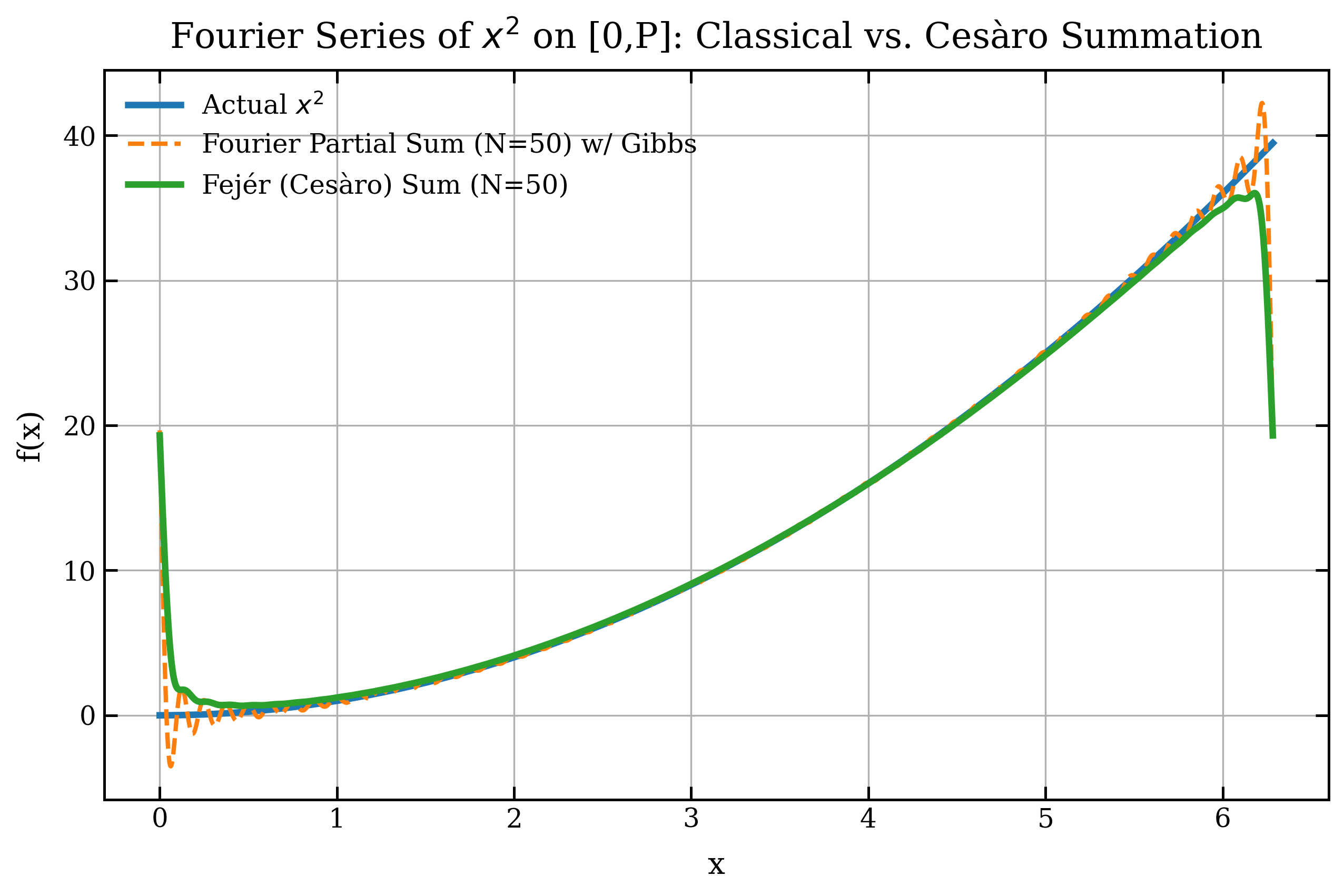
This page demonstrates Fourier series expansion and the Cesàro (Fejér) summation method, which can reduce Gibbs phenomenon oscillations.

Fourier Series

For a function $f (x)$ with period $P$ (so the integration interval is $[0, P]$ ), the Fourier series is:

f (x) \sim \frac{a _{0}}{2} + n = 1 \sum \infty [a_{n} cos (\frac{2 nπ x}{P}) + b_{n} sin (\frac{2 nπ x}{P})]

where the coefficients are:

a_{0} = \frac{2}{P} \int_{0}^{P} f (x) d x

a_{n} = \frac{2}{P} \int_{0}^{P} f (x) cos (\frac{2 nπ x}{P}) d x

b_{n} = \frac{2}{P} \int_{0}^{P} f (x) sin (\frac{2 nπ x}{P}) d x

The factor of 2 inside the trig arguments matters. With basis $cos (2 nπ x / P)$ and $sin (2 nπ x / P)$ , the basis functions have period $P / n$ , the fundamental period is $P$ , and the basis is orthogonal on $[0, P]$ with norm $P /2$ . That orthogonality is what makes the $(2/ P)$ normalization recover the coefficients exactly. If you instead use $cos (nπ x / P)$ on $[0, P]$ (period $2 P$ ), the sine and cosine families are no longer mutually orthogonal there, and the partial sum will not converge to $f$ .

Cesàro (Fejér) Summation

The classical partial sum $S_{N} (x)$ can exhibit Gibbs phenomenon near discontinuities. The Cesàro sum averages the partial sums:

σ_{N} (x) = \frac{1}{N + 1} k = 0 \sum N S_{k} (x)

This averaging reduces oscillations and provides better convergence behavior.

Implementation

The following code computes Fourier coefficients using the trapezoidal rule and compares classical and Cesàro summation:

import numpy as np
import matplotlib.pyplot as plt
import matplotlib as mpl

def set_publication_style():
    """Set publication-quality matplotlib style."""
    mpl.rcParams.update({
        'font.family': 'serif',
        'font.size': 12,
        'axes.labelsize': 14,
        'axes.titlesize': 16,
        'axes.linewidth': 1.2,
        'axes.labelpad': 8,
        'axes.titlepad': 10,
        'xtick.labelsize': 12,
        'ytick.labelsize': 12,
        'xtick.direction': 'in',
        'ytick.direction': 'in',
        'xtick.top': True,
        'ytick.right': True,
        'xtick.major.size': 6,
        'ytick.major.size': 6,
        'xtick.major.width': 1.2,
        'ytick.major.width': 1.2,
        'legend.fontsize': 12,
        'legend.frameon': False,
        'lines.linewidth': 2,
        'lines.markersize': 6,
        'figure.dpi': 100,
        'savefig.dpi': 300,
        'savefig.bbox': 'tight'
    })

set_publication_style()

# -------- PARAMETERS --------
P = 2*np.pi   # interval length
N = 50        # highest Fourier mode
M = 20000     # grid for trapezoidal rule

# -------- FUNCTION --------
def f(x):
    return x**2

# Grid for integration
x_int = np.linspace(0, P, M)
fx = f(x_int)

# -------- COMPUTE FOURIER COEFFICIENTS --------
a = np.zeros(N+1)
b = np.zeros(N+1)

# a0
a[0] = (2/P) * np.trapz(fx, x_int)

# n >= 1
for n in range(1, N+1):
    a[n] = (2/P) * np.trapz(fx * np.cos(2*n*np.pi * x_int/P), x_int)
    b[n] = (2/P) * np.trapz(fx * np.sin(2*n*np.pi * x_int/P), x_int)

# -------- BUILD CLASSICAL FOURIER PARTIAL SUM S_N(x) --------
x_plot = np.linspace(0, P, 2000)
S = np.zeros((N+1, len(x_plot)))

# S_0 = a0/2
S[0, :] = a[0]/2

for k in range(1, N+1):
    S[k, :] = S[k-1, :] + a[k] * np.cos(2*k*np.pi*x_plot/P) + b[k] * np.sin(2*k*np.pi*x_plot/P)

S_N = S[N, :]  # classical partial sum

# -------- CESÀRO (FEJÉR) SUM: sigma_N = (1/(N+1)) * sum_{k=0}^N S_k --------
sigma_N = np.sum(S, axis=0) / (N+1)

# -------- PLOT RESULTS --------
plt.figure(figsize=(10, 6))
plt.plot(x_plot, x_plot**2, label="Actual $x^2$", linewidth=3)
plt.plot(x_plot, S_N, '--', label=f"Fourier Partial Sum (N={N}) w/ Gibbs")
plt.plot(x_plot, sigma_N, label=f"Fejér (Cesàro) Sum (N={N})", linewidth=3)
plt.xlabel("x")
plt.ylabel("f(x)")
plt.title("Fourier Series of $x^2$ on [0,P]: Classical vs. Cesàro Summation")
plt.grid(True)
plt.legend()
plt.savefig('figures/fourier_series_cesaro.png', dpi=300, bbox_inches='tight')
plt.show()

Visualization

The following plot shows the Fourier series approximation with and without Cesàro summation:

Key Features

Fourier coefficient computation using trapezoidal rule
Classical partial sum construction
Cesàro summation for reduced oscillations
Comparison of convergence behavior

C++ Implementation

The following C++ code implements Fourier coefficient calculation with a functor-based design:

#include <functional>
#include <vector>
#include <numbers>
#include <cmath>
#include <iostream>

// Helper function: linspace
std::vector<double> linspace(double start, double end, size_t num) {
    std::vector<double> result(num);
    double dx = (end - start) / (num - 1);
    for (size_t i = 0; i < num; ++i) {
        result[i] = start + i * dx;
    }
    return result;
}

// Fourier basis functions
namespace sp {
    struct fourierSine {
        int n;
        double P;
        fourierSine(int n_, double P_) : n(n_), P(P_) {}
        double operator()(double x) {
            double pi = std::numbers::pi_v<double>; 
            return std::sin(2.0*n * pi * x / P);
        }
    };

    struct fourierCosine {
        int n;
        double P;
        fourierCosine(int n_, double P_) : n(n_), P(P_) {}
        double operator()(double x) {
            double pi = std::numbers::pi_v<double>; 
            return std::cos(2.0*n * pi * x / P);
        }
    };
}

// Trapezoidal rule template
template<typename F>
double trap(F f, double a, double b, int N) {
    double h = (b - a) / N;
    double s = 0.5 * (f(a) + f(b));
    for (int i = 1; i < N; ++i)
        s += f(a + i*h);
    return s * h;
}

// Inner product of two functions
double innerProduct(std::function<double(double)> f, 
                    std::function<double(double)> g, 
                    double a, double b, int N) {
    auto integrand = [&f, &g](double x) {
        return f(x) * g(x);
    };
    return trap(integrand, a, b, N);
}

// Fourier coefficient calculations
double a0Fourier(std::function<double(double)> f, double P, int n, int N) {
    return 2.0/P * trap(f, 0.0, P, N);
}

double aFourier(std::function<double(double)> f, double P, int n, int N) {
    auto cos_wrapper = sp::fourierCosine(n, P);
    return 2.0/P * innerProduct(f, cos_wrapper, 0.0, P, N);
}

double bFourier(std::function<double(double)> f, double P, int n, int N) {
    auto sin_wrapper = sp::fourierSine(n, P);
    return 2.0/P * innerProduct(f, sin_wrapper, 0.0, P, N);
}

// Fourier interpolant class
struct fourierInterp {
    std::vector<double> an;
    std::vector<double> bn;
    double a0;
    double L;
    
    fourierInterp(std::vector<double> an_, 
                  std::vector<double> bn_, 
                  double a0_, 
                  double L_)
        : an(an_), bn(bn_), a0(a0_), L(L_) {}

    double operator()(double x) {
        double result = a0 / 2.0;
        double pi = std::numbers::pi_v<double>; 
        
        for (int i = 0; i < an.size(); i++) {
            int n = i + 1;
            result += an[i]*std::cos(2.0*n * pi * x / L) 
                    + bn[i]*std::sin(2.0*n * pi * x / L);
        }
        return result;
    }
};

// Example usage
int main() {
    // Define function to approximate: f(x) = x^2
    auto f = [](double x){ return x*x; };
    
    double L = 6.28;  // Period
    int num_coeffs = 20;
    int integration_points = 20000;
    
    // Compute coefficients
    double a0 = a0Fourier(f, L, 1, integration_points);
    std::vector<double> a(num_coeffs);
    std::vector<double> b(num_coeffs);
    
    for(int n = 0; n < num_coeffs; n++) {
        a[n] = aFourier(f, L, n+1, integration_points);
        b[n] = bFourier(f, L, n+1, integration_points);
    }
    
    // Create interpolant
    fourierInterp finterp(a, b, a0, L);
    
    // Evaluate on grid
    std::vector<double> xs = linspace(0, L, 1000);
    std::vector<double> ys(xs.size());
    for(int i = 0; i < xs.size(); i++) {
        ys[i] = finterp(xs[i]);
    }
    
    // Print some results
    std::cout << "a0 = " << a0 << std::endl;
    std::cout << "First few coefficients:" << std::endl;
    for(int i = 0; i < 5; i++) {
        std::cout << "a[" << i+1 << "] = " << a[i] 
                  << ", b[" << i+1 << "] = " << b[i] << std::endl;
    }
    
    return 0;
}