Gradient Descent

Optimization

Gradient descent is the workhorse algorithm for minimizing differentiable functions. It shows up everywhere on this site that something gets minimized iteratively: neural-network training, logistic regression, variational energy minimization in Hartree-Fock, Newton-like residual iteration in finite elements, maximum-likelihood estimation in statistics. It's not an ML idea — it's a numerical-methods idea that ML uses constantly.

The recipe is one line. Pick a function $f : R^{n} \to R$ you want to minimize, pick a starting point $x_{0}$ , and iterate:

x_{k + 1} = x_{k} - η \nabla f (x_{k})

Two ingredients: the gradient (you compute or auto-differentiate it) and the step size $η$ (you pick it). Run until something stops changing. That's the whole algorithm. The interesting questions are all about why this works, when it doesn't, and how to set $η$ .

Why follow the negative gradient

At any point $x$ , the gradient $\nabla f (x)$ is the direction of steepest increase — the one that gives the biggest first-order rise in $f$ per unit step. The negative gradient is therefore steepest descent. Take a small step that way and you're guaranteed to decrease $f$ at first order:

f (x - η \nabla f) \approx f (x) - η ∥\nabla f ∥^{2} + O (η^{2})

The first-order term is negative as long as $\nabla f \neq = 0$ , so small enough $η$ always makes progress. The catch is in the $O (η^{2})$ — second-order curvature is what limits how big $η$ can be before the first-order improvement is wiped out by overshooting.

The step size

For a quadratic $f (x) = \frac{1}{2} x^{⊤} A x$ with positive-definite $A$ having largest eigenvalue $L$ , gradient descent converges if and only if $η < 2/ L$ . Above that, the iteration amplifies error in the worst-conditioned direction and diverges. Below, the contraction rate per step in direction $i$ is $∣1 - η λ_{i} ∣$ , so you converge as a geometric sequence with rate dominated by the worst eigenvalue.

For general smooth $f$ , the same logic applies locally — $L$ is the largest eigenvalue of the Hessian at the current point (or, more precisely, the Lipschitz constant of $\nabla f$ in the region you're moving through). Conservative practitioners use $η = 1/ L$ ; aggressive ones push to $η \approx 1.9/ L$ and zigzag toward the answer. Going past $2/ L$ diverges.

Demo: learning rate on an ill-conditioned bowl

Let's see this on a specific function. Take $f (x, y) = (x - 3)^{2} + 25 (y - 1)^{2}$ . The Hessian is $diag (2, 50)$ — eigenvalues 2 and 50, condition number 25. Stable learning rates are $η < 2/50 = 0.04$ . Try three:

Three panels showing gradient descent paths on (x-3)² + 25(y-1)² at learning rates 0.005, 0.035, and 0.041. The first crawls slowly along the y=1 axis. The second zigzags but converges. The third diverges with growing y-oscillations.

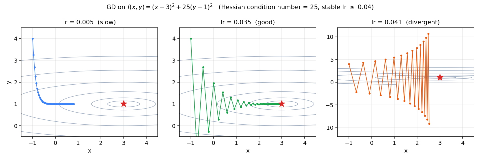
Left, $η = 0.005$ . The $y$ direction has contraction $∣1 - 0.005 \cdot 50∣ = 0.75$ , so $y$ snaps to 1 almost immediately. The $x$ direction has contraction $∣1 - 0.005 \cdot 2∣ = 0.99$ — barely under 1 — so $x$ crawls. After 60 iterations $x$ has covered about half the gap. Slow.

Middle, $η = 0.035$ . The $y$ contraction is now $∣1 - 0.035 \cdot 50∣ = 0.75$ — oscillating, but contracting fast. The $x$ contraction is $∣1 - 0.035 \cdot 2∣ = 0.93$ . After 60 iterations we're essentially at the minimum. Good, with visible zigzag near the steep direction.

Right, $η = 0.041$ . Just past the stability boundary. $∣1 - 0.041 \cdot 50∣ = 1.05$ — each $y$ -step grows by 5%. The $x$ component still converges (slowly), but $y$ spirals outward. Divergent.

This is the central frustration with vanilla gradient descent: the step size is constrained by the worst-conditioned direction, but progress is rate-limited by the best-conditioned direction. The ratio is the Hessian condition number $κ = L / μ$ , and convergence takes $O (κ lo g 1/ ε)$ iterations to reach error $ε$ . Loss landscapes from real ML problems often have $κ \sim 1 0^{6}$ — that's where momentum, preconditioners, Newton's method, and adaptive schemes (Adam, RMSprop) earn their keep.

Convex vs non-convex

For convex $f$ , every local minimum is a global minimum. GD with stable $η$ converges to the unique optimum from anywhere. For non-convex $f$ , GD finds a stationary point — but which one depends on where you started.

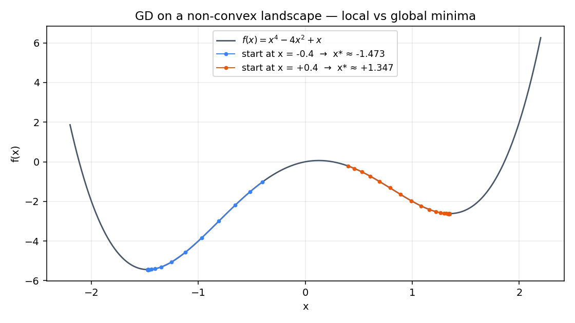
Plot of f(x) = x⁴ - 4x² + x with two basins of attraction. A trajectory starting at x = -0.4 falls into the left basin (local minimum near x = -1.47). A trajectory starting at x = +0.4 falls into the right basin (global minimum near x = +1.35).

Same function, same step size, two starting points 0.8 apart. One ends at $x \approx - 1.47$ (local minimum, $f \approx - 5.46$ ); the other ends at $x \approx + 1.35$ (global minimum, $f \approx - 2.66$ ). Gradient descent doesn't know there's a better basin. It rolls downhill from wherever you put it.

Standard practical responses: random restarts (try many starting points, keep the best), stochastic gradients (the noise helps escape shallow basins — this is half the reason SGD generalizes better than full-batch GD in deep learning), or methods that are explicitly global (simulated annealing, evolutionary search, Bayesian optimization). For convex problems none of this matters — gradient descent is enough.

Worked example: gradient descent reproduces OLS

The linear-regression page solves $\hat{β} = (X^{⊤} X)^{- 1} X^{⊤} y$ in closed form. The same answer comes out of gradient descent on the squared loss $L (β) = \frac{1}{n} ∥ y - Xβ ∥^{2}$ , whose gradient is $\nabla L (β) = - \frac{2}{n} X^{⊤} (y - Xβ)$ .

Mean-squared-error loss as a function of gradient descent iteration, on a log scale. The loss decays exponentially over the first ~20 iterations and then sits flat at the OLS optimum (red dashed line). 200 total iterations.

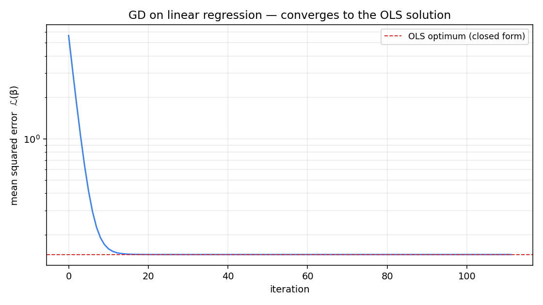
Loss is on a log scale. The exponential decay is the geometric convergence rate $(1 - η μ)^{k}$ for the $x^{⊤} X^{⊤} X x$ Hessian's smallest eigenvalue $μ$ . After 200 iterations the recovered coefficients match OLS to $4 \times 1 0^{- 11}$ — same answer, just iteratively. The closed-form solution is faster for this problem; GD wins when the design matrix is too big to factor.

The code

"""
Gradient descent demos.

Three figures + one text-output block:

  Fig 1: GD on an ill-conditioned 2D quadratic, three learning rates.
         Shows lr too small (slow), lr good (zigzag-but-converges),
         lr too big (divergent).

  Fig 2: GD on a non-convex 1D function. Two starting points → two
         different basins of attraction. Local-minimum behavior.

  Fig 3: Iterates of GD on the linear-regression squared loss recover
         the OLS coefficients from the closed-form normal equations.
"""

import numpy as np
import matplotlib.pyplot as plt


def gradient_descent(grad_f, x0, lr, n_iter, tol=1e-10):
    x = np.asarray(x0, dtype=float).copy()
    hist = [x.copy()]
    for _ in range(n_iter):
        g = np.asarray(grad_f(x), dtype=float)
        x = x - lr * g
        hist.append(x.copy())
        if np.linalg.norm(g) < tol:
            break
    return x, np.array(hist)


# ---------------------------------------------------------------------
# Demo 1: ill-conditioned 2D quadratic
#   f(x, y) = (x - 3)^2 + 25 (y - 1)^2
#   Hessian eigenvalues 2 and 50 → condition number 25.
#   Stable lr ≤ 2/L_max = 2/50 = 0.04.
# ---------------------------------------------------------------------

def f1(z):
    return (z[0] - 3.0) ** 2 + 25.0 * (z[1] - 1.0) ** 2

def grad_f1(z):
    return np.array([2.0 * (z[0] - 3.0), 50.0 * (z[1] - 1.0)])

x0 = np.array([-1.0, 4.0])
runs = []
for lr, label, n_it in [(0.005, "lr = 0.005  (slow)",        60),
                        (0.035, "lr = 0.035  (good)",        60),
                        (0.041, "lr = 0.041  (divergent)",   25)]:
    xf, hist = gradient_descent(grad_f1, x0, lr, n_it)
    runs.append((lr, label, xf, hist))


# ---------------------------------------------------------------------
# Demo 2: non-convex 1D, two basins
#   f(x) = x^4 - 4 x^2 + x
#   local min near x ≈ -1.5, global min near x ≈ 1.4
# ---------------------------------------------------------------------

def grad_f2(x):
    return np.array([4.0 * x[0] ** 3 - 8.0 * x[0] + 1.0])

starts = [-0.4, 0.4]
runs2 = [(x0_, *gradient_descent(grad_f2, [x0_], lr=0.03, n_iter=200))
         for x0_ in starts]


# ---------------------------------------------------------------------
# Demo 3: GD on the linear-regression squared loss.
# Same setup as Example 1 from the linear-regression page.
# Gradient: ∇ℒ(β) = -2/n Xᵀ(y - Xβ).
# Should recover the OLS estimate from the normal equations.
# ---------------------------------------------------------------------

rng = np.random.default_rng(42)
n  = 50
x  = rng.uniform(-2.0, 2.0, n)
y  = 0.5 + 2.0 * x + rng.normal(0.0, 0.5, n)
X  = np.column_stack([np.ones(n), x])
beta_ols = np.linalg.solve(X.T @ X, X.T @ y)

def grad_sq_loss(beta):
    return -2.0 * X.T @ (y - X @ beta) / n

beta_gd, hist3 = gradient_descent(
    grad_sq_loss, x0=np.array([0.0, 0.0]), lr=0.1, n_iter=200
)


# ---------------------------------------------------------------------
# Reporting
# ---------------------------------------------------------------------

print("Demo 1: ill-conditioned quadratic")
print("-" * 60)
for lr, label, xf, hist in runs:
    err = np.linalg.norm(xf - np.array([3.0, 1.0]))
    print(f"  {label:32s}   iters = {len(hist)-1:3d}   ‖x − x*‖ = {err:.3e}")
print()

print("Demo 2: non-convex 1D")
print("-" * 60)
for x0_, xf, hist in runs2:
    print(f"  start at x = {x0_:+.2f}   →   converged to x ≈ {xf[0]:+.4f}   ({len(hist)-1} iters)")
print()

print("Demo 3: GD recovers OLS")
print("-" * 60)
print(f"  OLS (closed form)   β = [{beta_ols[0]:+.4f}, {beta_ols[1]:+.4f}]")
print(f"  GD  (200 steps)     β = [{beta_gd[0]:+.4f}, {beta_gd[1]:+.4f}]")
print(f"  ‖β_ols − β_gd‖∞     = {np.abs(beta_ols - beta_gd).max():.2e}")

Running it

Demo 1: ill-conditioned quadratic
------------------------------------------------------------
  lr = 0.005  (slow)                 iters =  60   ‖x − x*‖ = 2.189e+00
  lr = 0.035  (good)                 iters =  60   ‖x − x*‖ = 5.141e-02
  lr = 0.041  (divergent)            iters =  25   ‖x − x*‖ = 1.017e+01

Demo 2: non-convex 1D
------------------------------------------------------------
  start at x = -0.40   →   converged to x ≈ -1.4730   (39 iters)
  start at x = +0.40   →   converged to x ≈ +1.3470   (56 iters)

Demo 3: GD recovers OLS
------------------------------------------------------------
  OLS (closed form)   β = [+0.4145, +2.0151]
  GD  (200 steps)     β = [+0.4145, +2.0151]
  ‖β_ols − β_gd‖∞     = 3.93e-11

When it works, when it doesn't

Works well when: the loss is convex (or near-convex around your starting point), the gradient is cheap to compute, the Hessian condition number isn't catastrophic, and you can pick a reasonable step size. This covers a surprisingly large fraction of real problems — linear/logistic regression, much of variational physics, MLE on well-posed likelihood functions.

Struggles when: the Hessian is severely ill-conditioned (you spend most iterations zigzagging across the wrong-direction valley), the loss is highly non-convex with many shallow local minima, the gradient is expensive (each iteration costs an entire MC chain or a full PDE solve), or you have constraints (gradient descent doesn't natively respect $x \geq 0$ or $g (x) = 0$ ). Each failure mode has a fix: momentum / preconditioning / Adam for ill-conditioning; stochastic restarts for non-convexity; quasi-Newton (BFGS) for expensive gradients; projected GD or Lagrangian methods for constraints. Most of those will get their own pages in this section.

Where this shows up on the site

Machine learning. Every iterative ML fit on the site uses gradient descent under the hood — linear regression (when the closed form isn't feasible), logistic regression (no closed form), neural networks (gradient through the chain rule, a.k.a. backpropagation). The ML-specific variants — SGD, momentum, Adam — are gradient descent with extra accounting and will live in the ML section since they're tied to deep-learning conventions.

Variational physics. The Hartree-Fock SCF iteration is fundamentally gradient descent on the orbital coefficients, minimizing $⟨ Φ∣ H ∣Φ ⟩$ subject to orthonormality. Variational Monte Carlo, density-functional minimization, geometry optimization in molecular dynamics — all gradient descent (often with quasi-Newton acceleration) on different energy functionals.

Numerical methods. Nonlinear residual iteration in finite elements, fitting parameters to time series, fitting potentials to atomistic data — all the same algorithm with different gradients plugged in.

Statistics. Maximum-likelihood estimation on any non-Gaussian likelihood (Poisson, multinomial, mixture models) usually reduces to gradient descent on $- lo g p (data ∣ θ)$ . Variational inference uses gradient descent on the ELBO.

Core idea

Gradient descent is "roll downhill in the steepest direction you can see." The math is one line. The art is picking a step size that respects the curvature of your loss surface in the worst direction, while not crawling in the best one. Every more advanced optimizer is some clever response to that tension.

Exercises

A full exercise set is available for this topic, structured as one worked example + 7 practice problems (across 7 surface contexts) + 2 pattern-resistant check problems.

Open the Gradient Descent exercise set → Pick a stable step size from the Hessian eigenvalues, run the iteration x ← x − η ∇f(x), and recognize the failure modes (divergence above 2/L, slow progress on ill-conditioned problems, traps on non-convex landscapes).

References

Nocedal, J., & Wright, S. (2006). Numerical Optimization, 2nd ed. Springer. Chapter 3 is the classical reference on step-size selection and line search.
Boyd, S., & Vandenberghe, L. (2004). Convex Optimization. Cambridge. Free PDF online. Chapter 9 covers gradient methods in the convex setting.
Bubeck, S. (2015). Convex Optimization: Algorithms and Complexity. Foundations and Trends in Machine Learning. Modern, ML-flavored treatment of convergence rates.
Polyak, B. T. (1987). Introduction to Optimization. Optimization Software. The classical Russian textbook; the source of "Polyak momentum."