Monte Carlo Option Pricing

Finance

Monte Carlo simulation is a powerful numerical method for pricing options, especially when analytical solutions are not available. It works by simulating many possible future stock price paths and averaging the payoffs.

Geometric Brownian Motion

We model the stock price $S_{t}$ using geometric Brownian motion:

d S_{t} = μ S_{t} d t + σ S_{t} d W_{t}

In the risk-neutral world, $μ = r$ . The solution is:

S_{t} = S_{0} exp ((r - \frac{σ ^{2}}{2}) t + σ W_{t})

For discrete time steps, we use:

S_{t + Δ t} = S_{t} exp ((r - \frac{σ ^{2}}{2}) Δ t + σ Δ t Z)

where $Z \sim N (0, 1)$ is a standard normal random variable.

Monte Carlo Method

The Monte Carlo method for option pricing:

Simulate $N$ stock price paths to expiration
Calculate the payoff for each path
Average the payoffs and discount to present value

The option price is estimated as:

V_{0} = e^{- r T} \frac{1}{N} i = 1 \sum N Payoff_{i}

The standard error decreases as $1/ N$ , so more simulations improve accuracy.

Payoff Functions

For a European call option:

Payoff = max (S_{T} - K, 0)

For a European put option:

Payoff = max (K - S_{T}, 0)

where $S_{T}$ is the stock price at expiration and $K$ is the strike price.

Python Implementation

The following code implements Monte Carlo option pricing:

import numpy as np
import matplotlib.pyplot as plt
import matplotlib as mpl
from scipy.stats import norm

def set_publication_style():
    """Set publication-quality matplotlib style."""
    mpl.rcParams.update({
        'font.family': 'serif',
        'font.size': 12,
        'axes.labelsize': 14,
        'axes.titlesize': 16,
        'axes.linewidth': 1.2,
        'axes.labelpad': 8,
        'axes.titlepad': 10,
        'xtick.labelsize': 12,
        'ytick.labelsize': 12,
        'xtick.direction': 'in',
        'ytick.direction': 'in',
        'xtick.top': True,
        'ytick.right': True,
        'xtick.major.size': 6,
        'ytick.major.size': 6,
        'xtick.major.width': 1.2,
        'ytick.major.width': 1.2,
        'legend.fontsize': 12,
        'legend.frameon': False,
        'lines.linewidth': 2,
        'lines.markersize': 6,
        'figure.dpi': 100,
        'savefig.dpi': 300,
        'savefig.bbox': 'tight'
    })

set_publication_style()

def black_scholes(S, K, T, r, sigma, option_type='call'):
    """Black-Scholes analytical formula for comparison."""
    d1 = (np.log(S / K) + (r + 0.5 * sigma**2) * T) / (sigma * np.sqrt(T))
    d2 = d1 - sigma * np.sqrt(T)
    
    if option_type == 'call':
        return S * norm.cdf(d1) - K * np.exp(-r * T) * norm.cdf(d2)
    else:
        return K * np.exp(-r * T) * norm.cdf(-d2) - S * norm.cdf(-d1)

def monte_carlo_option_price(S0, K, T, r, sigma, n_simulations, option_type='call', n_steps=1):
    """
    Price European option using Monte Carlo simulation.
    
    Parameters
    ----------
    S0 : float
        Initial stock price
    K : float
        Strike price
    T : float
        Time to expiration (years)
    r : float
        Risk-free rate
    sigma : float
        Volatility
    n_simulations : int
        Number of Monte Carlo simulations
    option_type : str
        'call' or 'put'
    n_steps : int
        Number of time steps (1 for simple simulation)
    
    Returns
    -------
    tuple
        Option price, standard error, payoffs array
    """
    np.random.seed(42)  # For reproducibility
    
    dt = T / n_steps
    
    # Simulate stock prices
    if n_steps == 1:
        # Simple one-step simulation
        Z = np.random.normal(0, 1, n_simulations)
        ST = S0 * np.exp((r - 0.5 * sigma**2) * T + sigma * np.sqrt(T) * Z)
    else:
        # Multi-step simulation
        ST = np.zeros(n_simulations)
        S = np.full(n_simulations, S0)
        
        for _ in range(n_steps):
            Z = np.random.normal(0, 1, n_simulations)
            S *= np.exp((r - 0.5 * sigma**2) * dt + sigma * np.sqrt(dt) * Z)
        
        ST = S
    
    # Calculate payoffs
    if option_type == 'call':
        payoffs = np.maximum(ST - K, 0)
    else:
        payoffs = np.maximum(K - ST, 0)
    
    # Discount to present value and calculate statistics
    option_price = np.exp(-r * T) * np.mean(payoffs)
    standard_error = np.exp(-r * T) * np.std(payoffs) / np.sqrt(n_simulations)
    
    return option_price, standard_error, payoffs

def simulate_stock_paths(S0, mu, sigma, T, dt, n_paths):
    """
    Simulate multiple stock price paths using geometric Brownian motion.
    
    Parameters
    ----------
    S0 : float
        Initial stock price
    mu : float
        Drift (expected return)
    sigma : float
        Volatility
    T : float
        Total time
    dt : float
        Time step
    n_paths : int
        Number of paths to simulate
    
    Returns
    -------
    ndarray
        Array of stock price paths
    """
    n_steps = int(T / dt)
    paths = np.zeros((n_paths, n_steps + 1))
    paths[:, 0] = S0
    
    for i in range(1, n_steps + 1):
        Z = np.random.normal(0, 1, n_paths)
        paths[:, i] = paths[:, i-1] * np.exp((mu - 0.5 * sigma**2) * dt + sigma * np.sqrt(dt) * Z)
    
    return paths

# Parameters
S0 = 100  # Initial stock price
K = 100   # Strike price
T = 1.0   # Time to expiration (1 year)
r = 0.05  # Risk-free rate (5%)
sigma = 0.2  # Volatility (20%)
n_simulations = 100000  # Number of Monte Carlo simulations

# Calculate option prices
call_price_mc, call_se, call_payoffs = monte_carlo_option_price(
    S0, K, T, r, sigma, n_simulations, 'call'
)
put_price_mc, put_se, put_payoffs = monte_carlo_option_price(
    S0, K, T, r, sigma, n_simulations, 'put'
)

# Compare with Black-Scholes
call_price_bs = black_scholes(S0, K, T, r, sigma, 'call')
put_price_bs = black_scholes(S0, K, T, r, sigma, 'put')

print("Monte Carlo Option Pricing Results:")
print("\nCall Option:")
print("  Monte Carlo: {:.4f} ± {:.4f}".format(call_price_mc, call_se))
print("  Black-Scholes: {:.4f}".format(call_price_bs))
print("  Difference: {:.4f}".format(abs(call_price_mc - call_price_bs)))
print("  Relative Error: {:.2f}%".format(100*abs(call_price_mc - call_price_bs)/call_price_bs))

print("\nPut Option:")
print("  Monte Carlo: {:.4f} ± {:.4f}".format(put_price_mc, put_se))
print("  Black-Scholes: {:.4f}".format(put_price_bs))
print("  Difference: {:.4f}".format(abs(put_price_mc - put_price_bs)))
print("  Relative Error: {:.2f}%".format(100*abs(put_price_mc - put_price_bs)/put_price_bs))

# Plot 1: Simulated stock price paths
n_paths_plot = 20
dt = 1/252  # Daily steps
paths = simulate_stock_paths(S0, r, sigma, T, dt, n_paths_plot)
time = np.linspace(0, T, paths.shape[1])

fig, axes = plt.subplots(2, 2, figsize=(14, 10))

# Top left: Stock price paths
axes[0, 0].plot(time, paths.T, alpha=0.6, linewidth=0.5)
axes[0, 0].axhline(K, color='r', linestyle='--', linewidth=2, label='Strike Price')
axes[0, 0].set_xlabel('Time (years)')
axes[0, 0].set_ylabel('Stock Price')
axes[0, 0].set_title('Simulated Stock Price Paths')
axes[0, 0].legend()
axes[0, 0].grid(True, alpha=0.3)

# Top right: Payoff distribution (call)
axes[0, 1].hist(np.exp(-r*T) * call_payoffs, bins=50, alpha=0.7, edgecolor='black')
axes[0, 1].axvline(call_price_mc, color='r', linestyle='--', linewidth=2, label='Mean: {:.2f}'.format(call_price_mc))
axes[0, 1].axvline(call_price_bs, color='g', linestyle='--', linewidth=2, label='BS: {:.2f}'.format(call_price_bs))
axes[0, 1].set_xlabel('Discounted Payoff')
axes[0, 1].set_ylabel('Frequency')
axes[0, 1].set_title('Call Option Payoff Distribution')
axes[0, 1].legend()
axes[0, 1].grid(True, alpha=0.3)

# Bottom left: Payoff distribution (put)
axes[1, 0].hist(np.exp(-r*T) * put_payoffs, bins=50, alpha=0.7, edgecolor='black', color='orange')
axes[1, 0].axvline(put_price_mc, color='r', linestyle='--', linewidth=2, label='Mean: {:.2f}'.format(put_price_mc))
axes[1, 0].axvline(put_price_bs, color='g', linestyle='--', linewidth=2, label='BS: {:.2f}'.format(put_price_bs))
axes[1, 0].set_xlabel('Discounted Payoff')
axes[1, 0].set_ylabel('Frequency')
axes[1, 0].set_title('Put Option Payoff Distribution')
axes[1, 0].legend()
axes[1, 0].grid(True, alpha=0.3)

# Bottom right: Convergence analysis
n_sims_range = [1000, 5000, 10000, 50000, 100000, 500000]
call_prices_conv = []
put_prices_conv = []

for n in n_sims_range:
    call_p, _, _ = monte_carlo_option_price(S0, K, T, r, sigma, n, 'call')
    put_p, _, _ = monte_carlo_option_price(S0, K, T, r, sigma, n, 'put')
    call_prices_conv.append(call_p)
    put_prices_conv.append(put_p)

axes[1, 1].semilogx(n_sims_range, call_prices_conv, 'b-o', label='Call (MC)')
axes[1, 1].semilogx(n_sims_range, put_prices_conv, 'r-o', label='Put (MC)')
axes[1, 1].axhline(call_price_bs, color='b', linestyle='--', alpha=0.5, label='Call (BS)')
axes[1, 1].axhline(put_price_bs, color='r', linestyle='--', alpha=0.5, label='Put (BS)')
axes[1, 1].set_xlabel('Number of Simulations')
axes[1, 1].set_ylabel('Option Price')
axes[1, 1].set_title('Monte Carlo Convergence')
axes[1, 1].legend()
axes[1, 1].grid(True, alpha=0.3)

plt.tight_layout()
plt.savefig('figures/monte_carlo_options_plot.png', dpi=300, bbox_inches='tight')
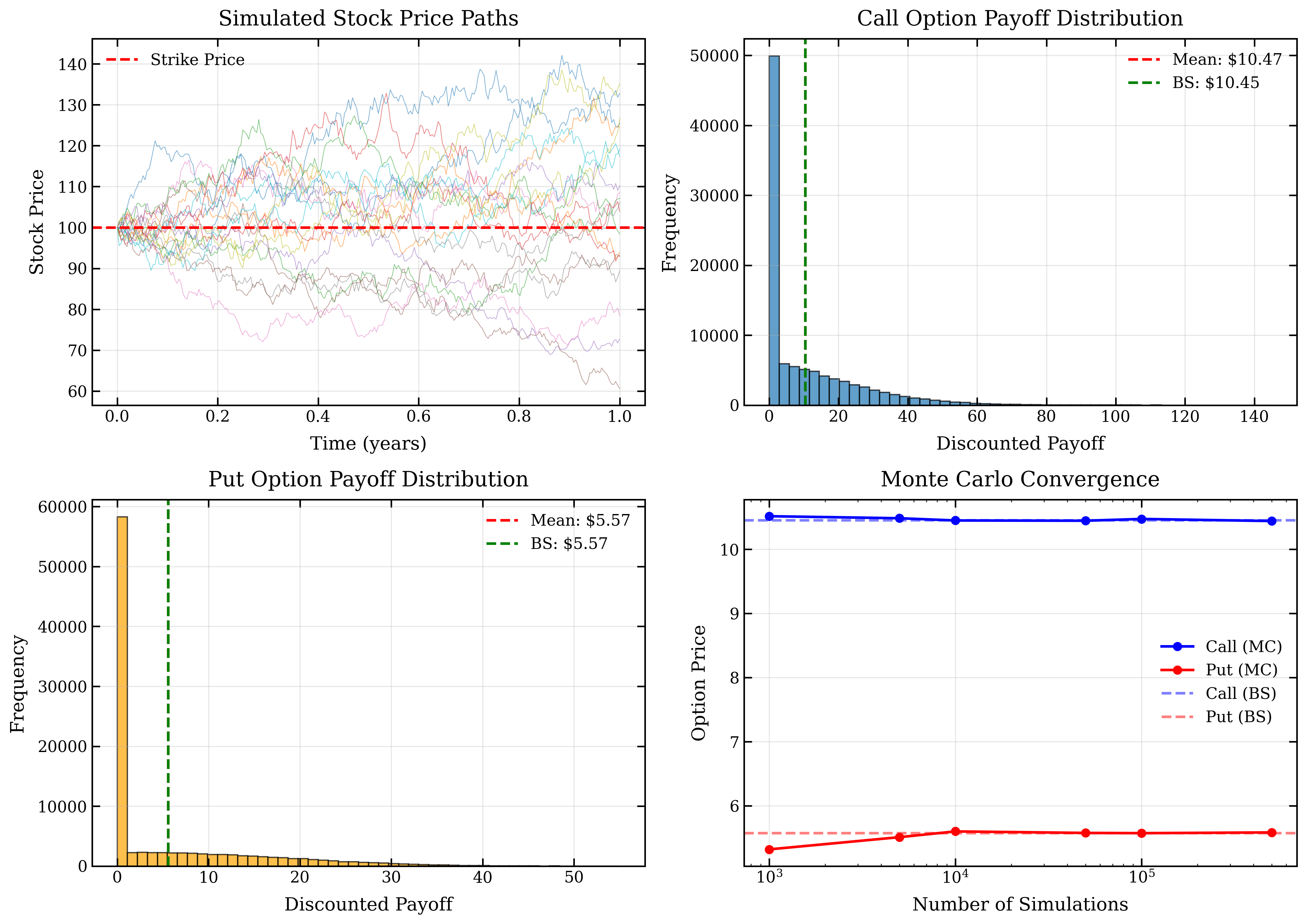
plt.show()

Visualization

The following plots show simulated stock price paths, payoff distributions, and convergence analysis:

Advantages

Monte Carlo simulation offers several advantages:

Flexibility: Can handle complex payoffs and path-dependent options
Multi-dimensional: Easy to extend to multiple assets
Stochastic volatility: Can incorporate time-varying volatility
American options: Can price early exercise using least squares Monte Carlo
Intuitive: Direct simulation of the underlying process

Variance Reduction

Several techniques can reduce the variance of Monte Carlo estimates:

Antithetic variates: Use $- Z$ along with $Z$
Control variates: Use known analytical solutions
Importance sampling: Change the probability measure
Quasi-Monte Carlo: Use low-discrepancy sequences

Applications

Monte Carlo is used for:

Exotic options (Asian, barrier, lookback)
Basket options and correlation products
Options with stochastic volatility
Real options and project valuation
Risk management and stress testing