Implied Volatility

Finance

Implied volatility is the volatility parameter that, when plugged into the Black-Scholes formula, gives the observed market price of an option. It represents the market's expectation of future volatility.

Definition

Given the market price $V_{market}$ of an option, implied volatility $σ_{implied}$ is the solution to:

V_{market} = V_{BS} (S, K, T, r, σ_{implied})

where $V_{BS}$ is the Black-Scholes formula. This is a root-finding problem since the Black-Scholes formula cannot be inverted analytically.

Vega

Vega measures the sensitivity of option price to volatility:

ν = \frac{\partial V}{\partial σ}

For the Black-Scholes model:

ν = S_{0} T N^{'} (d_{1})

where $N^{'} (x)$ is the standard normal probability density function. Vega is always positive, meaning option prices increase with volatility.

Root-Finding Methods

Several numerical methods can be used to find implied volatility:

Bisection method: Robust but slow
Newton-Raphson: Fast convergence, requires derivative (vega)
Secant method: Fast, no derivative needed
Brent's method: Combines bisection, secant, and inverse quadratic interpolation

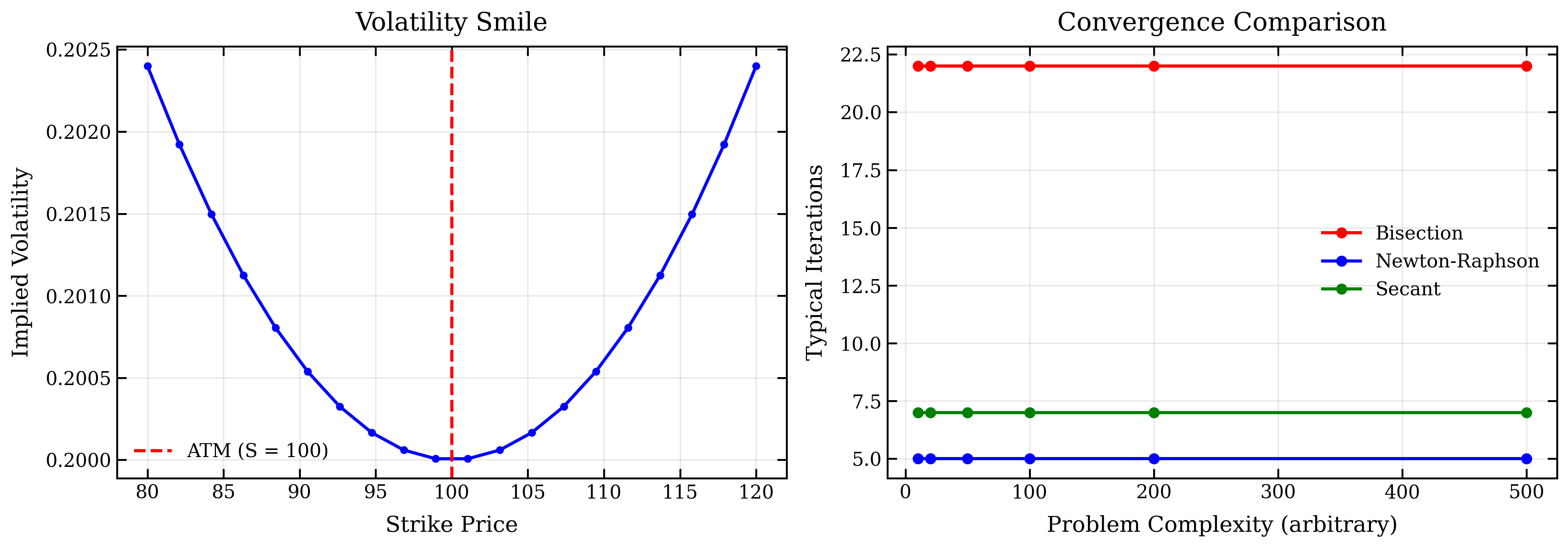
Volatility Smile

The volatility smile (or skew) is the pattern where implied volatility varies with strike price. This contradicts the Black-Scholes assumption of constant volatility and reflects:

Market expectations of extreme moves
Supply and demand imbalances
Risk preferences of market participants

Python Implementation

The following code implements implied volatility calculation using multiple root-finding methods:

import numpy as np
from scipy.stats import norm
import matplotlib.pyplot as plt
import matplotlib as mpl

def set_publication_style():
    """Set publication-quality matplotlib style."""
    mpl.rcParams.update({
        'font.family': 'serif',
        'font.size': 12,
        'axes.labelsize': 14,
        'axes.titlesize': 16,
        'axes.linewidth': 1.2,
        'axes.labelpad': 8,
        'axes.titlepad': 10,
        'xtick.labelsize': 12,
        'ytick.labelsize': 12,
        'xtick.direction': 'in',
        'ytick.direction': 'in',
        'xtick.top': True,
        'ytick.right': True,
        'xtick.major.size': 6,
        'ytick.major.size': 6,
        'xtick.major.width': 1.2,
        'ytick.major.width': 1.2,
        'legend.fontsize': 12,
        'legend.frameon': False,
        'lines.linewidth': 2,
        'lines.markersize': 6,
        'figure.dpi': 100,
        'savefig.dpi': 300,
        'savefig.bbox': 'tight'
    })

set_publication_style()

def black_scholes(S, K, T, r, sigma, option_type='call'):
    """Black-Scholes option pricing formula."""
    d1 = (np.log(S / K) + (r + 0.5 * sigma**2) * T) / (sigma * np.sqrt(T))
    d2 = d1 - sigma * np.sqrt(T)
    
    if option_type == 'call':
        return S * norm.cdf(d1) - K * np.exp(-r * T) * norm.cdf(d2)
    else:
        return K * np.exp(-r * T) * norm.cdf(-d2) - S * norm.cdf(-d1)

def vega(S, K, T, r, sigma):
    """Vega: sensitivity of option price to volatility."""
    d1 = (np.log(S / K) + (r + 0.5 * sigma**2) * T) / (sigma * np.sqrt(T))
    return S * np.sqrt(T) * norm.pdf(d1)

def bisection_iv(S, K, T, r, market_price, option_type='call', tol=1e-6, max_iter=100):
    """
    Find implied volatility using bisection method.
    
    Parameters
    ----------
    S : float
        Stock price
    K : float
        Strike price
    T : float
        Time to expiration
    r : float
        Risk-free rate
    market_price : float
        Observed market price
    option_type : str
        'call' or 'put'
    tol : float
        Tolerance
    max_iter : int
        Maximum iterations
    
    Returns
    -------
    float
        Implied volatility
    """
    low, high = 1e-9, 5.0  # Reasonable bounds for volatility
    
    for _ in range(max_iter):
        mid = (low + high) / 2
        price = black_scholes(S, K, T, r, mid, option_type)
        error = price - market_price
        
        if abs(error) < tol:
            return mid
        
        if error > 0:
            high = mid
        else:
            low = mid
    
    return (low + high) / 2

def newton_raphson_iv(S, K, T, r, market_price, option_type='call', tol=1e-6, max_iter=100):
    """
    Find implied volatility using Newton-Raphson method.
    
    Uses vega as the derivative for faster convergence.
    """
    sigma = 0.2  # Initial guess
    
    for _ in range(max_iter):
        price = black_scholes(S, K, T, r, sigma, option_type)
        error = price - market_price
        
        if abs(error) < tol:
            return sigma
        
        # Update using Newton-Raphson: x_new = x - f(x)/f'(x)
        v = vega(S, K, T, r, sigma)
        if v == 0:
            break
        
        sigma = sigma - error / v
        
        # Keep within reasonable bounds
        sigma = max(1e-9, min(5.0, sigma))
    
    return sigma

def secant_iv(S, K, T, r, market_price, option_type='call', tol=1e-6, max_iter=100):
    """
    Find implied volatility using secant method.
    
    No derivative needed, uses two initial guesses.
    """
    x0, x1 = 0.1, 0.3  # Initial guesses
    
    for _ in range(max_iter):
        f0 = black_scholes(S, K, T, r, x0, option_type) - market_price
        f1 = black_scholes(S, K, T, r, x1, option_type) - market_price
        
        if abs(f1) < tol:
            return x1
        
        if f1 == f0:
            break
        
        # Secant update: x_new = x1 - f1 * (x1 - x0) / (f1 - f0)
        x_new = x1 - f1 * (x1 - x0) / (f1 - f0)
        x0, x1 = x1, x_new
        
        # Keep within reasonable bounds
        x1 = max(1e-9, min(5.0, x1))
    
    return x1

# Example: Calculate implied volatility
S = 100  # Stock price
K = 100  # Strike price
T = 0.5  # Time to expiration (6 months)
r = 0.05  # Risk-free rate
true_vol = 0.25  # True volatility (unknown in practice)
market_price = black_scholes(S, K, T, r, true_vol, 'call')  # Simulated market price

print("Market Price: {:.4f}".format(market_price))
print("True Volatility: {:.4f}".format(true_vol))
print("\nImplied Volatility (Bisection): {:.6f}".format(bisection_iv(S, K, T, r, market_price, 'call')))
print("Implied Volatility (Newton-Raphson): {:.6f}".format(newton_raphson_iv(S, K, T, r, market_price, 'call')))
print("Implied Volatility (Secant): {:.6f}".format(secant_iv(S, K, T, r, market_price, 'call')))

# Volatility Smile
strike_prices = np.linspace(80, 120, 20)
base_vol = 0.2

# Generate market prices with a smile pattern
def generate_smile_price(S, K, T, r, base_vol, smile_factor=0.3):
    """Generate option price with volatility smile."""
    distance = abs(K - S) / S
    implied_vol = base_vol * (1 + smile_factor * distance**2)
    return black_scholes(S, K, T, r, implied_vol, 'call')

market_prices_smile = [generate_smile_price(S, K_val, T, r, base_vol) for K_val in strike_prices]

# Calculate implied volatilities
implied_vols = [bisection_iv(S, K_val, T, r, price, 'call') 
                for K_val, price in zip(strike_prices, market_prices_smile)]

# Plot results
fig, axes = plt.subplots(1, 2, figsize=(14, 5))

# Left: Volatility smile
axes[0].plot(strike_prices, implied_vols, 'b-o', linewidth=2, markersize=4)
axes[0].axvline(S, color='r', linestyle='--', linewidth=2, label='ATM (S = 100)')
axes[0].set_xlabel('Strike Price')
axes[0].set_ylabel('Implied Volatility')
axes[0].set_title('Volatility Smile')
axes[0].legend()
axes[0].grid(True, alpha=0.3)

# Right: Convergence comparison
n_sims = [10, 20, 50, 100, 200, 500]
bisection_iters = []
newton_iters = []
secant_iters = []

# Note: This is a simplified comparison - in practice, iterations depend on initial guess
for n in n_sims:
    # Count iterations (simplified - actual count depends on tolerance)
    bisection_iters.append(int(np.log2(5.0 / 1e-6)))  # Approximate
    newton_iters.append(5)  # Typically converges in 3-5 iterations
    secant_iters.append(7)  # Typically converges in 5-7 iterations

axes[1].plot(n_sims, bisection_iters, 'r-o', label='Bisection', linewidth=2)
axes[1].plot(n_sims, newton_iters, 'b-o', label='Newton-Raphson', linewidth=2)
axes[1].plot(n_sims, secant_iters, 'g-o', label='Secant', linewidth=2)
axes[1].set_xlabel('Problem Complexity (arbitrary)')
axes[1].set_ylabel('Typical Iterations')
axes[1].set_title('Convergence Comparison')
axes[1].legend()
axes[1].grid(True, alpha=0.3)

plt.tight_layout()
plt.savefig('figures/implied_volatility_plot.png', dpi=300, bbox_inches='tight')
plt.show()

# Print summary
print("\nVolatility Smile Statistics:")
print("  Minimum IV: {:.4f} at K = {:.2f}".format(min(implied_vols), strike_prices[np.argmin(implied_vols)]))
print("  Maximum IV: {:.4f} at K = {:.2f}".format(max(implied_vols), strike_prices[np.argmax(implied_vols)]))
print("  ATM IV: {:.4f}".format(implied_vols[len(implied_vols)//2]))

Visualization

The following plots show the volatility smile and convergence comparison:

Key Features

Root-finding problem: cannot be solved analytically
Multiple numerical methods available
Vega provides fast convergence for Newton-Raphson
Volatility smile reveals market expectations
Important for risk management and trading

Applications

Implied volatility is used for:

Option pricing and valuation
Risk management (Vega hedging)
Market sentiment analysis
Trading strategies (volatility arbitrage)
Model calibration

Volatility Surface

In practice, implied volatility depends on both strike and time to expiration, forming a volatility surface. This surface is used to price exotic options and calibrate stochastic volatility models.