“Know how to solve every problem that has been solved.” “What I cannot create, I do not understand.” — Richard Feynman

Black-Scholes Model

Finance

An option is a contract that gives its holder a choice later — a call is the right (not the obligation) to buy a stock at a fixed strike price $K$ on a fixed expiry date. What is that right worth today? Black and Scholes answered by changing the question: not "what will the stock do?" but "what does it cost to manufacture the option?" If a dealer can trade the stock continuously, she can build a portfolio that reproduces the option's payoff no matter where the stock goes — and then the option must cost what the manufacturing costs, or there is free money on the table. Every number on this page comes from code in this repository (scripts/gen_black_scholes.py), and the model's central claim is demonstrated below by simulation, not asserted.

The idea before any equations

Sell a call option and you are exposed: if the stock rises, you owe the difference. But the option's value moves with the stock — when the stock rises $1, the call rises by some fraction $Δ$ (between 0 and 1, called the option's delta). So hold $Δ$ shares against the short option, and over the next instant the two movements cancel. The combined book — short one option, long $Δ$ shares — is momentarily riskless, and a riskless position must earn exactly the risk-free interest rate $r$ (what a bank deposit pays), or arbitrage exists. Writing "the hedged book earns $r$ " in calculus produces the Black-Scholes equation. The hedge has to be adjusted as the stock moves and time passes — that continual adjustment is delta hedging, and its cost is the option's price.

One consequence surprises everyone the first time: the stock's expected return never appears. Whether the stock drifts up 8% a year or down 3%, the hedge cancels the direction and only the wiggle size — the volatility $σ$ — survives into the price. The simulation below runs the stock at an 8% drift while the formula knows only the 5% risk-free rate, and the hedge works anyway.

The model's world

The stock price $S_{t}$ is modeled as geometric Brownian motion: in each instant $d t$ the price changes by a predictable piece plus a coin-flip piece,

d S_{t} = μ S_{t} d t + σ S_{t} d W_{t}

where $μ$ is the drift (average growth rate), $σ$ is the volatility (the size of the random wiggles, quoted per year), and $d W_{t}$ is the coin flip — an increment of Brownian motion, a random step of typical size $d t$ . Both terms scale with $S_{t}$ itself, so it is percentage changes that are random — a $200 stock jumps twice as many dollars as a $100 stock. Solving this (Itô's lemma) gives a lognormal price:

S_{t} = S_{0} exp ((μ - \frac{σ ^{2}}{2}) t + σ W_{t})

For pricing, the hedging argument lets us set $μ = r$ — the so-called risk-neutral world. This is not a claim that stocks really drift at the risk-free rate; it is the mathematical shadow of the fact that the hedge cancels the drift, so we may price as if it were $r$ .

The equation and the formula

"The hedged book earns $r$ ", written out for an option value $C (S, t)$ , is a partial differential equation:

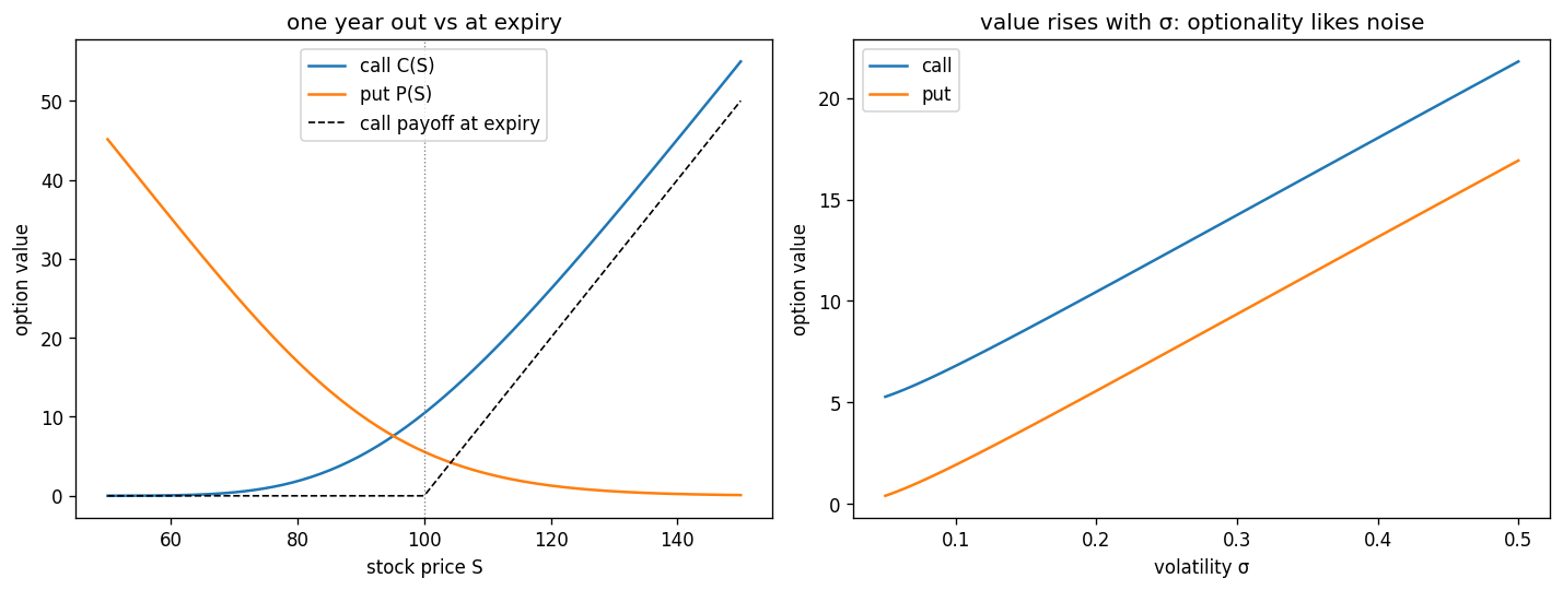
\frac{\partial C}{\partial t} + \frac{1}{2} σ^{2} S^{2} \frac{\partial ^{2} C}{\partial S ^{2}} + r S \frac{\partial C}{\partial S} - r C = 0

with the terminal condition that at expiry the option equals its payoff, $C (S, T) = max (S - K, 0)$ for a call. For European options (exercisable only at expiry) the PDE has a closed-form solution:

C = S_{0} N (d_{1}) - K e^{- r T} N (d_{2}), P = K e^{- r T} N (- d_{2}) - S_{0} N (- d_{1})

d_{1} = \frac{ln ( S _{0} / K ) + ( r + σ ^{2} /2 ) T}{σ T}, d_{2} = d_{1} - σ T

Here $N (x)$ is the standard normal cumulative distribution function — the probability that a standard Gaussian lands below $x$ . The two terms read like a story: $N (d_{2})$ is the (risk-neutral) probability the option finishes in the money, so $K e^{- r T} N (d_{2})$ is the discounted strike you expect to pay, and $S_{0} N (d_{1})$ is the value of the stock you expect to receive, with $d_{1} > d_{2}$ because receiving the stock is worth more on exactly the paths where the stock ended high.

Left: call and put values against stock price one year from expiry, with the kinked call payoff for comparison. Right: both option values rising with volatility. — Left: option values one year out (smooth) against the payoff at expiry (kinked) — time and volatility round the kink off. Right: value rises with $σ$ ; an option holder owns the upside of the noise but not the downside, so more noise is worth more.

Checking it three ways

All checks run in scripts/gen_black_scholes.py with $S_{0} = K = 100$ , $T = 1$ year, $r = 5%$ , $σ = 20%$ . First, price the same call two independent ways — the closed form, and 200,000 simulated risk-neutral paths:

closed form call  C = 10.450584
Monte Carlo call    = 10.463414 +/- 0.033118   (0.39 SE away)
parity: C - P = 4.877057549929   S - K e^-rT = 4.877057549929   diff = 0.00e+00

The Monte Carlo agrees within a third of its own standard error, and put-call parity — the model-independent identity $C - P = S - K e^{- r T}$ , which must hold for European options or a static arbitrage exists — holds to the last printed digit.

The third check is the one that matters, because it tests the argument rather than the algebra. Sell one call at the formula price, delta-hedge it at $N$ evenly spaced times, and settle at expiry. The stock paths are simulated with a real-world 8% drift — not the 5% the formula uses — so this also tests the claim that the drift drops out:

rehedges N   std of hedge P&L   (short 1 call, premium 10.45)
        4     3.1890
       16     1.6688
       64     0.8498
      256     0.4241
     1024     0.2148
log-log slope = -0.488   (theory: -0.5)
unhedged short call: std = 16.645;  hedged (N=64): std = 0.843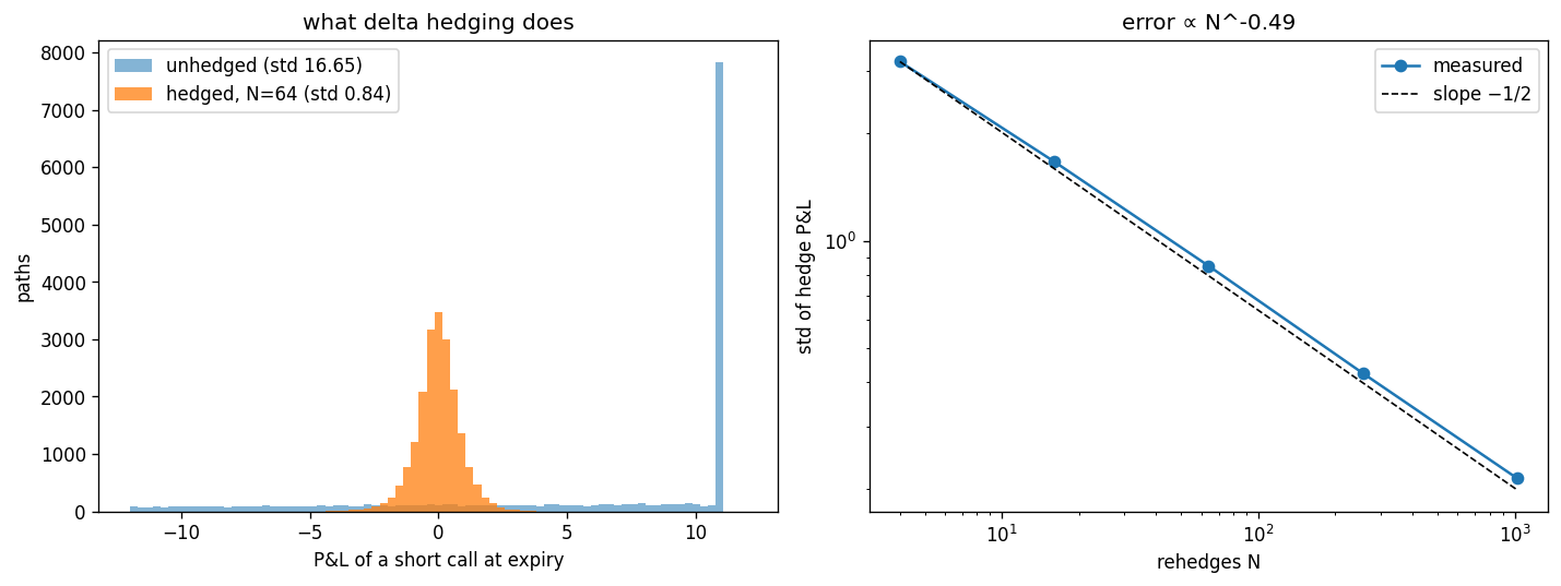

Left: P&L histogram of a short call, unhedged (wide, with a spike at full premium) vs delta-hedged at 64 rebalances (narrow peak at zero). Right: log-log plot of hedge P&L standard deviation against number of rehedges, following the slope minus one half line. — Left: the P&L of a short call across 20,000 paths. Unhedged, it is a gamble — the spike at +10.45 is every path where the option died worthless and the seller kept the premium; the long left tail is where it did not. Hedged 64 times, the same book collapses to a peak at zero (std 16.6 → 0.84, a 20× reduction). Right: the residual error falls as $N^{- 1/2}$ — measured slope −0.488 against the theoretical −½. Continuous hedging is the $N \to \infty$ limit in which the option is manufactured exactly.

That last plot is the Black-Scholes model: the price is fair precisely because the payoff can be manufactured, and the manufacturing error is controlled by how often you rebalance. The $1/ N$ rate has the same origin as the standard error of a mean — each rehedging interval contributes an independent $O (d t)$ slice of unhedged randomness, and $N$ independent slices average down like $N$ .

The pricing function

import numpy as np
from scipy.stats import norm

def black_scholes(S, K, T, r, sigma, option_type="call"):
    d1 = (np.log(S / K) + (r + 0.5 * sigma**2) * T) / (sigma * np.sqrt(T))
    d2 = d1 - sigma * np.sqrt(T)
    if option_type == "call":
        return S * norm.cdf(d1) - K * np.exp(-r * T) * norm.cdf(d2)
    return K * np.exp(-r * T) * norm.cdf(-d2) - S * norm.cdf(-d1)

print(black_scholes(100, 100, 1.0, 0.05, 0.20, "call"))   # 10.450584
print(black_scholes(100, 100, 1.0, 0.05, 0.20, "put"))    #  5.573526

The sensitivities of this function — delta, gamma, theta, vega, rho — are the Greeks, and they have their own page with working code: Greeks and delta hedging.

Where the model breaks

The formula assumes one volatility for all strikes and expiries. Markets disagree: back out the $σ$ that reproduces each traded option price and you get the volatility smile — different implied volatilities at different strikes, the subject of the implied volatility and volatility surface pages. Real returns also have fatter tails than the lognormal allows: the October 1987 crash was a ~20-standard-deviation event under GBM, which is the polite way of saying the distributional assumption failed, and the smile appeared in equity markets immediately afterward. The model survives these failures because of how it is used in practice: as a quoting convention (prices are quoted in implied volatility) and as the base case more realistic models are measured against.

Notation: one formula, five costumes

Derivatives pricing has a notation problem: every major textbook writes the same objects differently, and the differences look like math when they are only spelling. This page uses $C (S, t)$ , $N (\cdot)$ for the standard normal CDF, and $d_{1}, d_{2}$ . Here is the translation table for reading anything else:

object	here / Hull	Shreve	Wilmott	papers/desks
option value	$C, P$	$c (t, x)$	$V (S, t)$	$f$ , $u$
normal CDF	$N (x)$	$Φ (x)$	$N (x)$	$N, Φ$
the two arguments	$d_{1}, d_{2}$	$d_{\pm}$	$d_{1}, d_{2}$	$d_{\pm}$
Brownian motion	$d z$	$d W (t)$	$d X$	$d W_{t}, d B_{t}$
risk-neutral expectation	"risk-neutral world"	$\tilde{E}$	—	$E^{Q}$

Two of the differences are genuine traps, not just spelling. First, time: some books work in calendar time $t$ , others in time-to-expiry $τ = T - t$ — and since $\partial / \partial t = - \partial / \partial τ$ , the theta of an option flips sign depending on the convention. A "positive theta" claim means nothing until you know which clock the author is holding. Second, carry: Hull writes the dividend yield $q$ explicitly, Black-76 replaces the spot with the forward $F$ (absorbing $r$ and $q$ at once), and older texts use the cost-of-carry $b$ where $b = r$ is stock, $b = r - q$ is dividend-paying, $b = 0$ is futures. Three parameterizations of one idea — and formulas copied between conventions without translating are the classic way to be silently wrong by a factor of $e^{q τ}$ .

The defense is the one this page practices: declare the convention once, then translate at the border. When a formula from another source disagrees with yours, check the clock and the carry before suspecting the math.

References

F. Black and M. Scholes, J. Political Economy 81, 637 (1973); R. C. Merton, Bell J. Econ. 4, 141 (1973) — the hedging argument as presented here is closer to Merton's. J. Hull, Options, Futures, and Other Derivatives for the practitioner's treatment; S. Shreve, Stochastic Calculus for Finance II for the measure-theoretic one.