Linear-Response Analysis of LIF Networks via Lanczos+CF

A network of leaky integrate-and-fire neurons is exactly linear between spikes: the membrane equation $\tau dv/dt=-v+Wv+bu(t)$ is a linear ODE in the vector $v$ of subthreshold voltages, with $W$ a sparse synaptic-coupling matrix. So computing "how does the network respond to a small input at neuron 0, measured at neuron $i$, at frequency $\omega$?" is the same problem as the circuit-MOR problem — a resolvent matrix element of a giant sparse symmetric operator. On the right kind of network, Lanczos plus continued fraction converges to machine precision in tens of iterations, on systems where direct frequency-sweep solves take seconds and a full-cortex-scale model would take days.

What $H(\omega )$ means, and why compute it

Before the math: $H(\omega )$ is the frequency-resolved gain of the network at one neuron when that neuron is driven by an oscillating current. Three regimes:

• At $\omega =0$ (DC): the steady-state voltage per unit DC current — the network's input resistance as seen from that neuron. Different from the bare single-cell input resistance because recurrent feedback adds (or subtracts) effective conductance.
• At large $\omega$: the membrane averages the input over its time constant; response decays as $1/\omega$.
• At intermediate $\omega$: peaks in $|H(\omega )|$ are network resonances — the frequencies the network amplifies. Pole locations come from the imaginary parts of $L$'s eigenvalues; widths come from the eigenvectors' overlap with the input.

For a single passive LIF neuron, $H(\omega )=1/(1+i\omega \tau )$ — a boring low-pass filter. The interesting structure comes from the recurrent matrix $W$: collective modes appear as poles of $H(\omega )$, the Ritz values produced by the Lanczos chain.

Five reasons someone in a neuroscience lab actually does this calculation:

1. Predicting experimental responses. Inject an oscillating current into a brain slice, or shine flickering light onto an animal at frequency $\omega$. Linear response says: the response amplitude is $|H(\omega )|$ times the input. This is how transcranial alternating-current stimulation (tACS) entrains a brain rhythm — drive at the frequency where $H(\omega )$ peaks.
2. Validating models against measured power spectra. EEG / MEG / LFP recordings produce time series whose power spectrum, under standard noise-driven assumptions, is proportional to $|H(\omega ){|}^2$. If a model's $H(\omega )$ doesn't reproduce the measured $1/f^{\alpha }$ or peaked spectra, the model is wrong somewhere — connectivity, time constants, or excitatory-inhibitory balance.
3. Detecting proximity to instability. As ${\lambda }_{\max }(W)\to 1$ the network approaches a synchronous-oscillatory transition. $H(\omega )$ develops a sharp resonance peak whose height and width quantify how close the system is to the transition. This is the math behind "critical brain" arguments (Beggs-Plenz neuronal avalanches, edge-of-chaos computation).
4. Reading off the network's natural rhythms. The poles of $H(\omega )$ are the eigenvalues of $L$. Lanczos gives them as Ritz values, and the continued fraction packages them as the rational function's structure. Computing $H(\omega )$ extracts the network's eigenfrequencies for free.
5. Cross-region signal propagation. Off-diagonal $H_{ij}(\omega )=e_j^{\mathsf{T}}(s1-L{)}^{-1}{e}_i$ gives "drive at $i$, response at $j$ at frequency $\omega$." The matrix $H(\omega )$ over all pairs is the network's frequency-dependent communication map — directly relevant to how information propagates through connectomes (e.g., DTI-derived structural networks).

The single-port $H(\omega )$ we'll compute below is the simplest case. The architecture of the calculation — sparse linear operator, resolvent matrix element, Lanczos+CF — extends directly to the off-diagonal cases with separate input and output starting vectors. Same machinery, more outputs.

The model and its linear-response operator

Take $N$ rate-coupled LIF units, each with membrane time constant $\tau$. Stack the subthreshold voltages into a vector $v(t)\in {\mathbb{R}}^N$. The equation

has $W$ as the synaptic-coupling matrix (entry $W_{ij}$ is the synaptic strength from neuron $j$ onto neuron $i$), and $b$ as the input vector localizing an external drive $u(t)$ to a particular neuron or set of neurons. In the Laplace domain:

The transfer function from a current injection at neuron 0 to the voltage at neuron 0 is then

A single matrix element of the resolvent of the linear-response operator $L$, just as in TDDFT, VLSI MOR, and DMFT. Set $A=-L$ (positive-definite provided ${\lambda }_{\max }(W)<1$, which is the asynchronous-irregular stability condition) and the resolvent becomes a Lanczos+CF problem at shift $z=-s$.

Demo

Build a sparse symmetric coupling matrix $W$ on $N=400$ neurons with 8% density and coupling $g=0.6$ (below the Sommers-Crisanti-Sompolinsky instability threshold). Drive at neuron 0, read at neuron 0, sweep $\omega \in [1,10^4]$ rad/s.

# Lanczos + continued-fraction analysis of a sparse linearized LIF network.
# tau dv/dt = -v + W v + b u(t)
# Linearized dynamics operator:  L = (-I + W) / tau
# Transfer function (single port at neuron 0):
#   H(s) = b^T (s I - L)^{-1} b
# Compute H(j omega) two ways: direct sparse solve, and Lanczos+CF.

import numpy as np
import scipy.sparse as sp
import scipy.sparse.linalg as spla

N = 400
tau = 1e-2          # 10 ms
sparsity = 0.08
g = 0.6             # coupling — keep below spectral-radius threshold

rng = np.random.default_rng(42)
mask = rng.random((N, N)) < sparsity
W = (rng.standard_normal((N, N)) / np.sqrt(sparsity * N)) * g * mask
W = (W + W.T) / 2.0
np.fill_diagonal(W, 0.0)
W = sp.csr_matrix(W)
I_N = sp.eye(N)
L  = (-I_N + W) / tau
A  = -L              # symmetric positive-definite

port = 0
b = np.zeros(N); b[port] = 1.0
v0 = b.copy()        # unit norm

def lanczos(A, v0, n_iter):
    a, bt, Q = [], [], [v0.copy()]
    q_prev = np.zeros_like(v0); q = v0.copy(); beta_prev = 0.0
    for j in range(n_iter):
        w = A @ q
        alpha = float(q @ w)
        w = w - alpha * q - beta_prev * q_prev
        for qk in Q[:-1]:
            w -= float(qk @ w) * qk
        beta = float(np.linalg.norm(w))
        a.append(alpha)
        if beta < 1e-14: break
        if j < n_iter - 1:
            bt.append(beta); q_prev = q; q = w / beta
            Q.append(q.copy())
    return np.array(a), np.array(bt)

def cf(a, b_, z):
    f = a[-1] - z
    for j in range(len(a) - 2, -1, -1):
        f = (a[j] - z) - b_[j] ** 2 / f
    return 1.0 / f

# Direct frequency sweep
omegas = np.logspace(0, 4, 60)
H_direct = np.array([
    b @ spla.spsolve((1j * w * I_N - L).tocsc(), b) for w in omegas
])

# One Lanczos chain, evaluate continued fraction at every frequency.
alphas, betas = lanczos(A, v0, n_iter=80)
def H_lanczos(n, s):
    return cf(alphas[:n], betas[:n - 1], -s)

print(f"  {'chain':>6}   {'max relative error':>22}")
rel_norm = np.max(np.abs(H_direct))
for n in [10, 20, 40, 80]:
    H_n = np.array([H_lanczos(n, 1j * w) for w in omegas])
    err = np.max(np.abs(H_direct - H_n)) / rel_norm
    print(f"  {n:>6}   {err:>22.3e}")

   chain     max relative error
      10              4.861e-06
      20              1.961e-11
      40              7.467e-16
      80              7.467e-16

Read the table top-to-bottom: chain length 10 gives 5 parts per million, chain length 20 gives 2 parts per $10^{11}$, chain length 40 hits machine precision. Doubling the chain length roughly squares the error — that is geometric Padé convergence in its purest form, exactly as the Heine-Markov-Stieltjes theorem predicts when the spectrum of $A$ is well-conditioned.

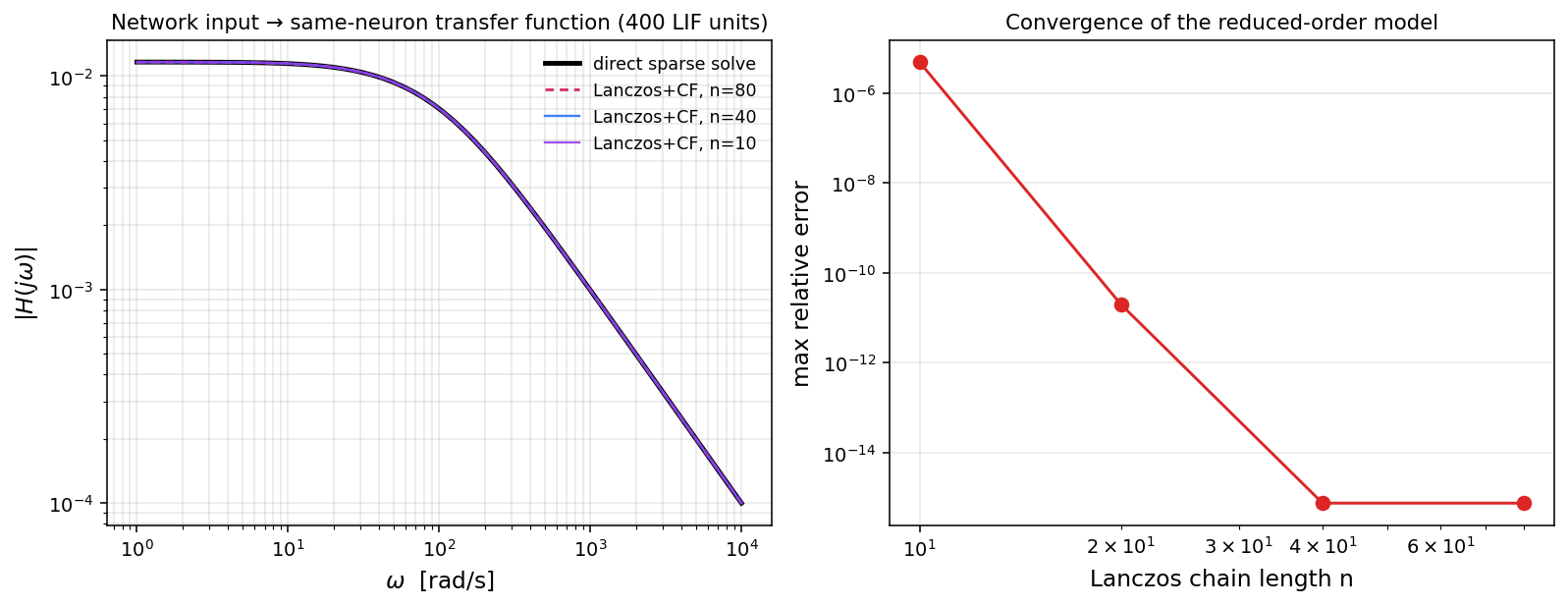
The four transfer-function curves on the left overlap to within line thickness — even the $n=10$ truncation is visually indistinguishable from direct. The right panel makes the convergence rate quantitative: geometric, hitting machine precision at $n=40$.

Why convergence is so fast here

The key fact is the spectrum of $W$. For a random matrix with sparsity $p$ and zero-mean entries of variance ${\sigma }^2/pN$, the spectral radius is $\sigma$ in the large-$N$ limit (Sommers-Crisanti-Sompolinsky 1988 for the asymmetric case, Wigner 1958 for the symmetric one). With our $g=0.6$ we get ${\lambda }_{\max }(W)\approx 0.85$, safely below 1.

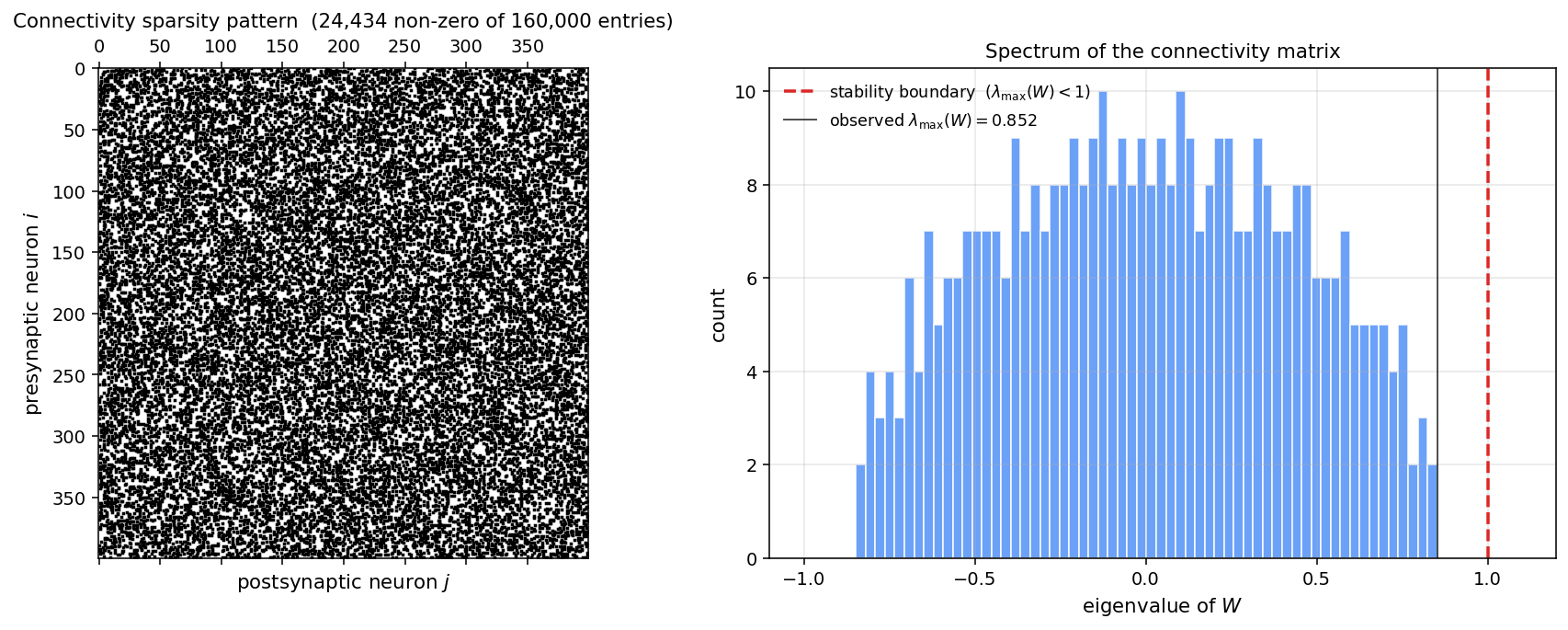
Translate to $A=-L=(1-W)/\tau$: with $\tau =10$ ms, the eigenvalues of $A$ live in $[(1-0.85)/\tau ,(1+0.85)/\tau ]\approx [15,185]$, one decade of spread. Compare to the RC ladder on the circuits page, whose spectrum of $K$ spanned nine decades. The classical estimate is that $n$ Lanczos iterations resolve eigenvalues to relative accuracy $\sim (\sqrt{\kappa }/(\sqrt{\kappa }+1){)}^n$, where $\kappa ={\lambda }_{\max }/{\lambda }_{\min }$ is the condition number. Here $\kappa \approx 12$ so the rate is $\approx 0.77$ per iteration — squaring the precision every five iterations. The numerics in the table match that rate almost exactly.

What about the spike-reset?

The demo above treats $v$ as a continuous subthreshold variable. Real LIF dynamics include a discontinuity: when $v_i$ crosses threshold the neuron emits a spike and $v_i$ resets. That nonlinear event breaks the strict linearity of the ODE.

Three standard reformulations bring the spike-reset back inside linear-response theory:

• Diffusion approximation (Brunel 2000). In the asynchronous-irregular regime, the population input to each neuron is approximately Gaussian white noise around a mean. The single-neuron equation becomes a Fokker-Planck PDE for the membrane-voltage density. Linearize this PDE around the stationary state; the linearized population-firing-rate response to a small perturbation IS a resolvent matrix element of the linearized Fokker-Planck operator. Lanczos+CF applies directly.
• Spike-train as a linear filter of the input. Treat the firing as a Poisson process whose intensity depends linearly on the filtered membrane voltage. The whole input-to-firing-rate map is then linear under this approximation.
• Population-density approach (Knight 1972; Omurtag-Knight-Sirovich 2000). Evolve a probability density $\rho (v,t)$ on the membrane-voltage axis with reset-at-threshold as a boundary condition. The resulting evolution operator is linear in $\rho$. Resolvent matrix elements of that operator give population firing-rate transfer functions.

All three reformulations end up at the same kind of resolvent matrix element of a sparse linear operator, with Lanczos+CF as the natural solver. The literature on linearized LIF networks (Brunel-Hakim 1999, Brunel 2000, Mattia-Del Giudice 2002, Lindner-Schimansky-Geier 2004) is in effect a long sequence of these constructions, applied in different limits.

Scale and limits

For symmetric $W$ the demo above generalizes straightforwardly. Real cortical connectivity is generally asymmetric (Dale's law forbids a neuron from being both excitatory and inhibitory, so $W_{ij}$ and $W_{ji}$ are constrained to have the same sign on the same row but different rows have different signs). For asymmetric $W$ the coupled-Lanczos chain becomes the bi-orthogonal Lanczos recurrence and the continued fraction is still well-defined, with the same Padé-equivalence theorem — just with separate left and right Krylov chains.

Scale estimates: a cortical microcircuit (one cortical column, $\sim 10^5$ neurons, sparse $\sim 10\%$ connectivity) gives a sparse matrix with $\sim 10^9$ non-zero entries. Direct factorization is prohibitive; matrix-free Lanczos+CF is the right tool. A whole-cortex model ($10^9$-$10^{10}$ neurons) requires further reduction — typically mean-field collapse to a much smaller set of population-density operators, then the same Lanczos+CF machinery on the reduced system. The Brunel network analysis used in BlueBrain and SpiNNaker pipelines is exactly this layered reduction.

Where this fits

Same Krylov+continued-fraction machinery as everything else on this site, applied to a sparse symmetric linear-response operator on a brain network. The mathematical structure shared with Casida-equation TDDFT, Liouville-Lanczos for solids, VLSI interconnect MOR, and Anderson-impurity DMFT solvers is exact — the operator changes, the algorithm doesn't. For LIF networks the spectrum is naturally well-conditioned (one decade of spread in the bulk), which is why the same algorithm that struggled on the nine-decade RC ladder converges geometrically here.

Related on this site

• Leaky integrate-and-fire (single neuron) — the single-unit model underlying everything on this page.
• Lanczos MOR for large circuits — same machinery on a network of RLC elements; the ill-conditioned counterpoint to this page's well-conditioned example.
• Lanczos iteration — the underlying algorithm and the Padé-via-Lanczos correspondence.
• Bi-orthogonal Lanczos — the non-symmetric variant needed for asymmetric (Dale-law) cortical connectivity.
• Liouville-Lanczos for TDDFT — the physics analog: resolvent matrix elements of a linear operator on a giant sparse problem.