“Know how to solve every problem that has been solved.” “What I cannot create, I do not understand.” — Richard Feynman

Lanczos + Continued Fractions for Circuit Model-Order Reduction

Circuits

Modern chips have millions to billions of parasitic R, L, and C nodes from the metal-interconnect layout. To run AC analysis or transient simulation, you'd want the frequency response of the network — but the matrix is too big to factor at every frequency, or even once. This is the classic setting for model-order reduction: replace the giant network with a small rational approximation of its transfer function that's accurate over the band of interest. The standard industrial algorithms — AWE, PVL, PRIMA — all rest on the same mathematical correspondence we demonstrated on the Lanczos iteration page: a Krylov chain on a sparse symmetric matrix produces a continued-fraction expansion of any resolvent matrix element. This page applies that correspondence to a concrete circuit and shows where the easy version works, where it fails, and what industrial codes do about it.

The math: MNA as a resolvent

Modified Nodal Analysis (MNA) writes the Kirchhoff equations of a linear circuit at frequency $s = jω$ as

(G + s C) v (s) = b (s),

where $G$ is the conductance matrix (from resistors and other algebraic constraints), $C$ is the capacitance matrix, $v$ is the vector of node voltages, and $b$ is the source vector. For a purely passive RC network, $G$ and $C$ are symmetric positive-semidefinite — they're quadratic forms coming from dissipated power and stored energy respectively.

Pick an input port (driven by $b$ ) and an output port (read out by some projection vector $l$ ). The transfer function from input to output is

H (s) = l^{T} (G + s C)^{- 1} b .

This is a matrix element of a resolvent. Same structural form as the dynamic polarizability in TDDFT or the impurity Green's function in DMFT — a giant sparse symmetric pencil and you want one element of its inverse as a function of $s$ .

Symmetrizing the pencil

The Lanczos-based continued fraction we built on the Lanczos page needs a single symmetric operator and a single starting vector. The pencil $(G, C)$ isn't immediately in that form. Fix: Cholesky-factor the capacitance matrix as $C = L L^{T}$ (for diagonal $C$ , $L$ is just $C$ ). Then

G + s C = L (K + s I) L^{T}, K := L^{- 1} G L^{- T},

where $K$ is sparse, symmetric, and positive-definite. The transfer function becomes

H (s) = (L^{- 1} l)^{T} (K + s I)^{- 1} (L^{- 1} b) = ∥ L^{- 1} b ∥^{2} ⟨ v_{0} ∣ (K + s I)^{- 1} ∣ v_{0} ⟩,

for a single-port impedance (input = output) with $v_{0} = L^{- 1} b /∥ L^{- 1} b ∥$ . The impedance is a single diagonal element of the resolvent of $K$ . Lanczos on $K$ starting from $v_{0}$ gives the tridiagonal projection; the continued fraction in the Lanczos coefficients gives $H (s)$ at every $s$ .

Demo: an RC ladder

Concrete example. An RC ladder is a 1D chain: $N$ nodes, a series resistor between each neighboring pair, a shunt capacitor from each node to ground.

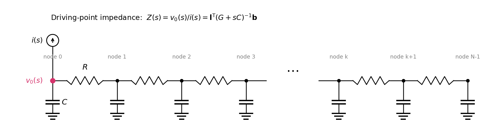
Schematic of an RC ladder: current source i(s) injected at node 0, series resistors R connecting consecutive nodes, capacitor C from each node to ground. The voltage v_0(s) at the injection node is the driving-point impedance Z(s) = v_0/i.

Drive a current source $i (s)$ at node 0 and read the voltage $v_{0} (s)$ at the same node. Their ratio is the driving-point impedance $Z (s) = v_{0} (s) / i (s)$ , which is exactly the resolvent matrix element we just wrote down. The "ground" symbols at the bottom of every capacitor are physically the chip's ground plane (one big shared zero-volt reference); mathematically they're the constraint that fixes one node of the network so the equations have a unique solution.

Here's the calculation done both ways:

# Lanczos + continued-fraction model-order reduction of an RC ladder.
# Compute Z(s) at one node, two ways:
#   (1) Direct sparse solve at every frequency.
#   (2) Single Lanczos chain on the symmetrized pencil + continued fraction.

import numpy as np
import scipy.sparse as sp
import scipy.sparse.linalg as spla

# 1D RC ladder: N nodes, series resistors between neighbors,
# capacitor to ground at each node, tiny leak for positive-definiteness.
N = 500
R_val = 1.0
C_val = 1.0e-9
g = 1.0 / R_val

diag = np.full(N, 2.0 * g); diag[0] = g; diag[-1] = g; diag += 1e-9
off  = np.full(N - 1, -g)
G    = sp.diags([off, diag, off], [-1, 0, 1], format='csr')
C_m  = sp.diags([C_val] * N, format='csr')

# Driving-point port at node 0.
b = np.zeros(N); b[0] = 1.0

# Symmetrize: G + sC = L (K + sI) L^T  with  L = sqrt(C).
# For diagonal C, L is diagonal too.
Linv = sp.diags(1.0 / np.sqrt(C_val * np.ones(N)))
K    = (Linv @ G @ Linv).tocsr()      # sparse, symmetric, positive-definite
bp   = Linv @ b
norm_bp = np.linalg.norm(bp)
v0   = bp / norm_bp

# Lanczos with full reorthogonalization.
def lanczos(A, v0, n_iter):
    alphas, betas, Q = [], [], [v0.copy()]
    q_prev = np.zeros_like(v0); q = v0.copy(); beta_prev = 0.0
    for j in range(n_iter):
        w = A @ q
        alpha = float(q @ w)
        w = w - alpha * q - beta_prev * q_prev
        for qk in Q[:-1]:
            w -= float(qk @ w) * qk
        beta = float(np.linalg.norm(w))
        alphas.append(alpha)
        if beta < 1e-14: break
        if j < n_iter - 1:
            betas.append(beta)
            q_prev = q; q = w / beta
            Q.append(q.copy())
    return np.array(alphas), np.array(betas)

def cf_eval(alphas, betas, z):
    """1 / ((alpha_0 - z) - beta_0^2 / ((alpha_1 - z) - ...))."""
    f = alphas[-1] - z
    for j in range(len(alphas) - 2, -1, -1):
        f = (alphas[j] - z) - betas[j] ** 2 / f
    return 1.0 / f

# Direct sweep
omegas = np.logspace(0, 10, 120)
Z_direct = np.array([
    np.dot(b, spla.spsolve((G + 1j * w * C_m).tocsc(), b))
    for w in omegas
])

# Single Lanczos chain — gives Z(s) at every frequency from the same coefficients.
alphas, betas = lanczos(K, v0, N)

def Z_lanczos(s, n):
    return norm_bp ** 2 * cf_eval(alphas[:n], betas[:n - 1], -s)

# Compare
for n in [10, 40, 160, N]:
    Z = np.array([Z_lanczos(1j * w, n) for w in omegas])
    rel_err = np.max(np.abs(Z - Z_direct)) / np.max(np.abs(Z_direct))
    print(f"chain length {n:>4}: max relative error = {rel_err:.3e}")

chain length   10: max relative error = 1.000e+00
chain length   40: max relative error = 1.000e+00
chain length  160: max relative error = 9.999e-01
chain length  500: max relative error = 1.231e-07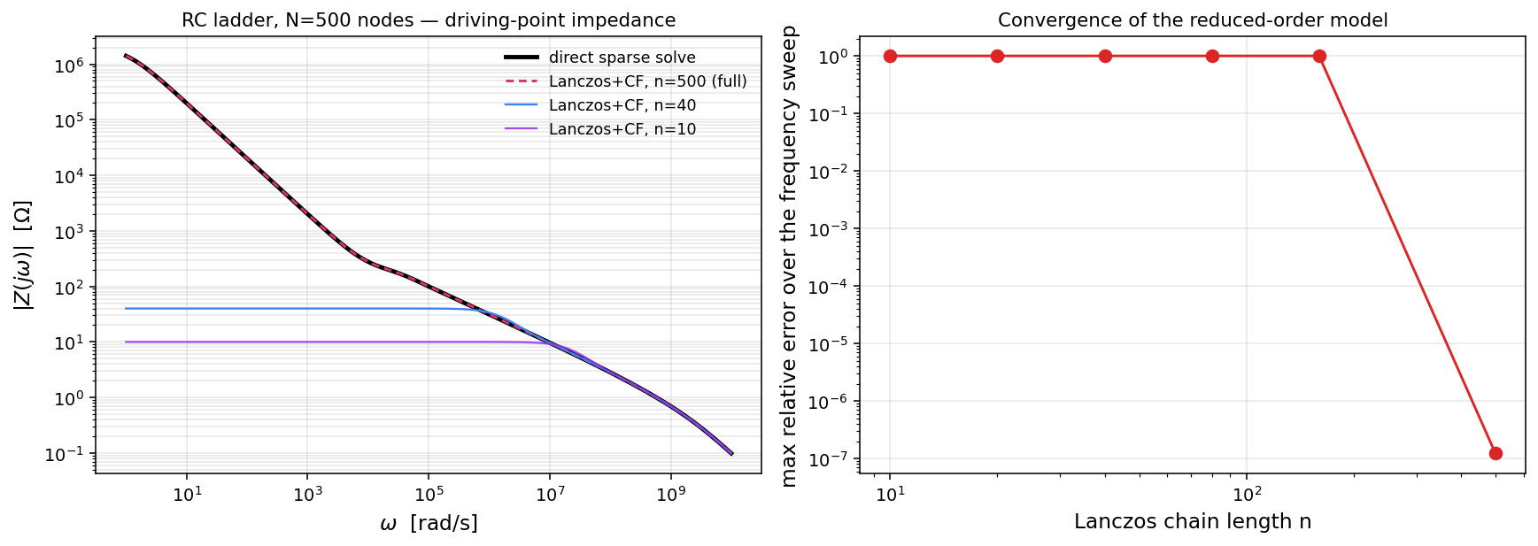

Left: |Z(jω)| for a 500-node RC ladder, computed by direct sparse solve (black) and Lanczos+CF at chain lengths 10, 40, and 500. Full chain overlays direct; short chains are flat at the high-frequency asymptote and miss the low-frequency resistive plateau. Right: convergence — max relative error stays at order 1 until the chain captures essentially the whole spectrum, then drops to 1e-7.

What this tells us

Two clean facts and one inconvenient one. Fact 1: the full chain ( $n = N = 500$ ) reproduces direct sparse solve to a relative accuracy of $1 0^{- 7}$ . The correspondence isn't approximate — Lanczos + continued fraction IS the resolvent matrix element when the chain runs to completion. Fact 2: the same chain gives $H (s)$ at every frequency, with no re-factorization. That's the speedup story when it works.

The inconvenient fact: the truncated chains are useless on this problem. $n = 40$ chain has 100% relative error; even $n = 160$ only gets to 99.99%. The next two subsections explain what's going on.

How the Padé approximant is actually formed

Time to derive it instead of name-dropping it. Work in terms of $K$ 's spectral decomposition. Eigenvalues $λ_{1}, λ_{2}, \dots, λ_{N}$ with orthonormal eigenvectors $∣ j ⟩$ , and decompose the (unit) starting vector as $v_{0} = \sum_{j} c_{j} ∣ j ⟩$ with $\sum_{j} ∣ c_{j} ∣^{2} = 1$ . The resolvent matrix element is, by direct insertion,

G (z) := ⟨ v_{0} ∣ (K - z 1)^{- 1} ∣ v_{0} ⟩ = j = 1 \sum N \frac{∣ c _{j} ∣ ^{2}}{λ _{j} - z} .

A sum of simple poles at the eigenvalues, weighted by the overlap of $v_{0}$ with each eigenmode. This function is the Stieltjes transform of the discrete measure $d μ (λ) = \sum_{j} ∣ c_{j} ∣^{2} δ (λ - λ_{j}) d λ$ . Define its moments

μ_{k} := \int λ^{k} d μ (λ) = j \sum ∣ c_{j} ∣^{2} λ_{j}^{k} = ⟨ v_{0} ∣ K^{k} ∣ v_{0} ⟩, k = 0, 1, 2, \dots

Two facts to notice. First, $μ_{0} = ∥ v_{0} ∥^{2} = 1$ . Second, every moment is computable as an inner product $v_{0}^{T} K^{k} v_{0}$ — you don't need eigenvalues or eigenvectors to get them.

The asymptotic expansion of $G (z)$ at infinity

Factor $- 1/ z$ out of each pole and expand the resulting geometric series, valid for $∣ z ∣ > max_{j} λ_{j}$ :

G (z) = - \frac{1}{z} j \sum ∣ c_{j} ∣^{2} \cdot \frac{1}{1 - λ _{j} / z} = - \frac{1}{z} j \sum ∣ c_{j} ∣^{2} k = 0 \sum \infty (\frac{λ _{j}}{z})^{k} = - k = 0 \sum \infty \frac{μ _{k}}{z ^{k + 1}} .

So at infinity,

G (z) = - \frac{μ _{0}}{z} - \frac{μ _{1}}{z ^{2}} - \frac{μ _{2}}{z ^{3}} - \dots = - \frac{1}{z} - \frac{⟨ K ⟩}{z ^{2}} - \frac{⟨ K ^{2} ⟩}{z ^{3}} - \dots

This is exact, term by term. Every coefficient $μ_{k} = ⟨ v_{0} ∣ K^{k} ∣ v_{0} ⟩$ is a moment of the underlying measure, and is directly computable from $K$ and $v_{0}$ .

What "Padé approximant" precisely means

The $[n - 1 / n]$ Padé approximant of $G (z)$ at infinity is the unique rational function

R_{n} (z) = \frac{P _{n - 1} ( z )}{Q _{n} ( z )}, de g P_{n - 1} = n - 1, de g Q_{n} = n,

whose own asymptotic expansion at $z = \infty$ agrees with $G (z)$ 's through as many terms as possible. Counting degrees of freedom: $Q_{n}$ contributes $n$ coefficients, $P_{n - 1}$ contributes $n$ more, overall normalization removes one, leaving $2 n - 1$ free coefficients. So the best you can do is match the first $2 n$ series coefficients of $G (z)$ :

R_{n} (z) = - \frac{μ _{0}}{z} - \frac{μ _{1}}{z ^{2}} - \dots - \frac{μ _{2 n - 1}}{z ^{2 n}} + O (\frac{1}{z ^{2 n + 1}}) .

So a Padé approximant isn't an arbitrary construction. It's the rational function that's correct on the first $2 n$ moments of the underlying measure. Doubling $n$ doubles how many moments you get right.

Multiply out the continued fraction explicitly

Now look at the truncated continued fraction with $n$ levels:

CF_{n} (z) = \frac{1}{( α _{0} - z ) - \frac{β _{0}^{2}}{( α _{1} - z ) - \frac{β _{1}^{2}}{⋱ - \frac{β _{n - 2}^{2}}{α _{n - 1} - z}}}} .

Do $n = 2$ by hand:

CF_{2} (z) = \frac{1}{( α _{0} - z ) - \frac{β _{0}^{2}}{α _{1} - z}} = \frac{α _{1} - z}{( α _{0} - z ) ( α _{1} - z ) - β _{0}^{2}} .

Numerator is degree 1 in $z$ , denominator is degree 2. A rational function $P_{1} (z) / Q_{2} (z)$ . Expand the denominator:

Q_{2} (z) = z^{2} - (α_{0} + α_{1}) z + (α_{0} α_{1} - β_{0}^{2}) .

Now compute the characteristic polynomial of the $2 \times 2$ Lanczos tridiagonal

T_{2} = (α_{0} β_{0} β_{0} α_{1}), det (T_{2} - z 1) = (α_{0} - z) (α_{1} - z) - β_{0}^{2} = z^{2} - (α_{0} + α_{1}) z + (α_{0} α_{1} - β_{0}^{2}) .

Identical to $Q_{2} (z)$ . So the denominator of $CF_{2}$ is $(- 1)^{2} = + 1$ times the characteristic polynomial of $T_{2}$ . Its two roots — the Ritz values of $T_{2}$ — are exactly the two poles of $CF_{2} (z)$ in $z$ .

The same algebra works at every order. Apply Cramer's rule for inverses of tridiagonal matrices to $(T_{n} - z 1)^{- 1}$ , expand the determinant along the first row, and the recursion collapses to the continued fraction. The result:

CF_{n} (z) = [(T_{n} - z 1)^{- 1}]_{0, 0} = \frac{det ( T _{n - 1} - z 1 )}{det ( T _{n} - z 1 )},

where $T_{n - 1}$ is the $(n - 1) \times (n - 1)$ submatrix of $T_{n}$ obtained by deleting the first row and column. So the poles of $CF_{n} (z)$ are the Ritz values — the eigenvalues of $T_{n}$ .

Why this rational function is the Padé approximant of $G (z)$

The deep step. The Lanczos coefficients $α_{j}, β_{j}$ aren't arbitrary numbers — they're the three-term-recurrence coefficients of the orthogonal polynomials with respect to the spectral measure $d μ$ of $v_{0}$ under $K$ :

\int p_{m} (λ) p_{n} (λ) d μ (λ) = δ_{mn}, λ p_{n} (λ) = β_{n} p_{n + 1} (λ) + α_{n} p_{n} (λ) + β_{n - 1} p_{n - 1} (λ) .

This three-term recurrence IS the Lanczos recurrence rewritten in polynomial language. Consequently the characteristic polynomial of $T_{n}$ equals $β_{0} β_{1} \dots β_{n - 1}$ times the $n$ -th orthogonal polynomial of the measure. Its $n$ roots — the Ritz values — are therefore the Gauss-quadrature nodes for $d μ$ .

The classical fact (Gauss, Christoffel, Stieltjes, Markov, 19th century, beautifully exposed in Trefethen & Bau's Numerical Linear Algebra Lecture 37 and Stahl-Totik's General Orthogonal Polynomials): an $n$ -point Gauss-quadrature rule for a measure on the real line matches the first $2 n$ moments of the measure exactly. Reading that statement through the Stieltjes-transform identity: the rational function whose poles are the Gauss-quadrature nodes and whose residues are the Gauss-quadrature weights agrees with $G (z)$ on the first $2 n$ coefficients of the asymptotic series at infinity. That's exactly the definition of the $[n - 1/ n]$ Padé approximant.

So three statements are the same statement:

Multiply out the $n$ -level Lanczos continued fraction; you get a rational function with poles at the Ritz values.
Build the $n$ -point Gauss-quadrature rule for the measure $d μ$ ; the nodes and weights produce a rational function approximating $G (z)$ .
Match the first $2 n$ coefficients of the asymptotic series of $G (z)$ at infinity with a rational function of type $[n - 1/ n]$ ; the result is uniquely determined.

All three give the same rational function. That's Heine, Markov, and Stieltjes's theorem from the 1880s-90s, predating Lanczos by half a century, and it's the reason "Padé approximant" and "Lanczos continued fraction" name the same object.

Practical consequence for our problem: the $n$ -th truncated continued fraction has $n$ poles. They sit at the $n$ Ritz values — the eigenvalues of $T_{n}$ . These poles are placed by the Gauss-quadrature theory: they pick out $n$ representative points of the spectrum, weighted in a way that makes the truncated rational function correct on the first $2 n$ moments.

Visualizing the failure

Now look at where those Ritz values actually sit on this problem. The plot below shows the true eigenvalues of $K$ at the top, and below them the Ritz values produced by Lanczos at chain lengths 4, 8, 16, 32, 64, and 100 (full chain for a smaller 100-node version of the ladder, kept smaller so the eigenvalues are individually visible).

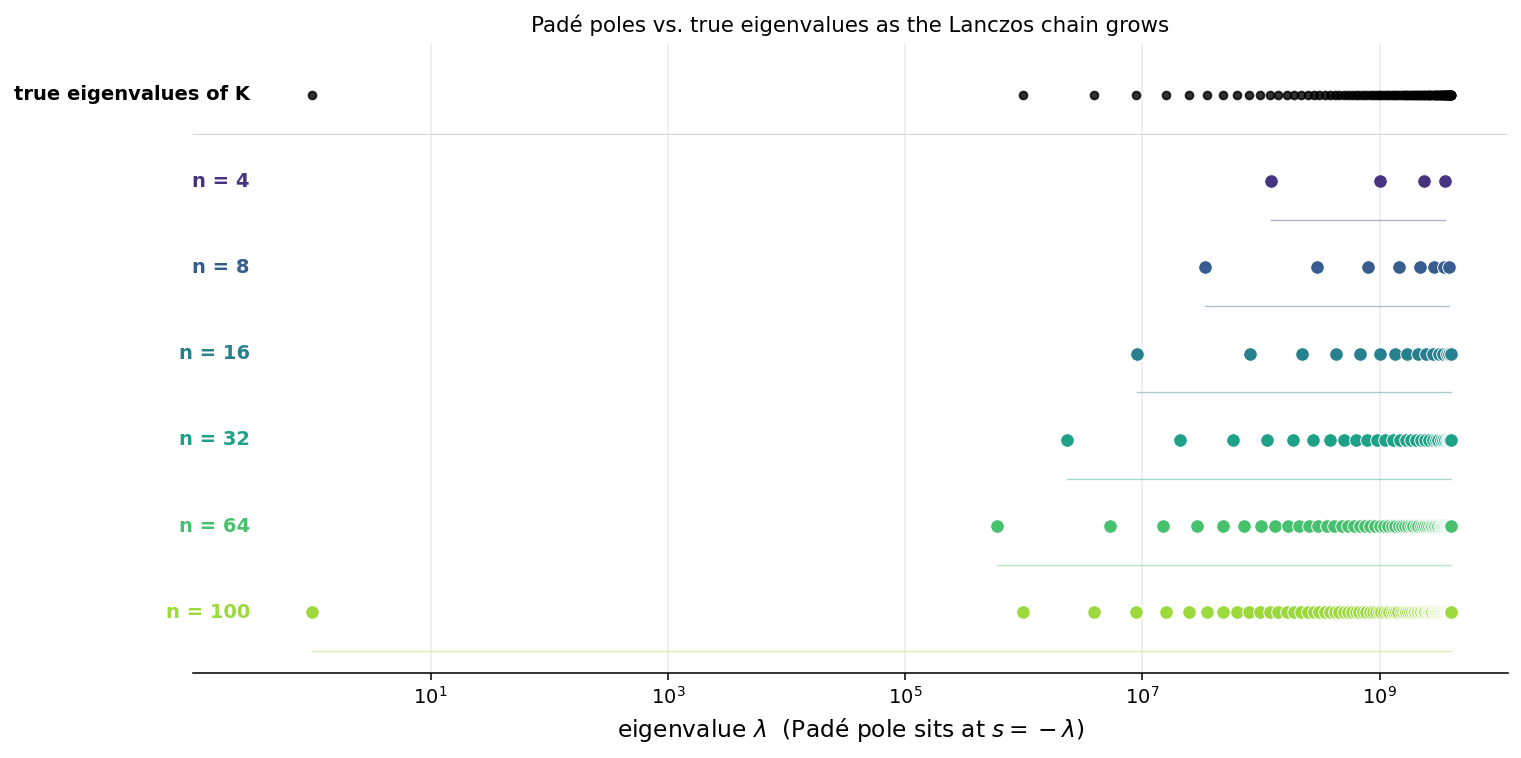
Top row: 100 true eigenvalues of K, one isolated near 1 and the rest in a band between 10^6 and 10^9. Lower rows: Ritz values for chain lengths 4, 8, 16, 32, 64, 100. Until n=100, the Ritz values cluster entirely in the upper band — none of them approximate the isolated small eigenvalue near 1.

Two things to see. First, the true eigenvalues of $K$ (top row) are spread across roughly nine orders of magnitude: one isolated eigenvalue sits near $λ \approx 1$ , and a dense band of the other 99 fills the range $λ \in [1 0^{6}, 4 \times 1 0^{9}]$ . That's what "the spectrum spans many decades" actually means — the eigenvalues are scattered across factors of $1 0^{9}$ in size, reflecting the physical fact that an RC ladder has time constants ranging from the smallest $RC$ (fastest local response, nanoseconds) to $N^{2} RC$ (slowest collective response, milliseconds for an N=100 ladder).

Second, the failure mode. Lanczos at $n = 4$ places its Padé poles entirely in the upper band — none of them sit near the isolated low-eigenvalue mode at $λ \approx 1$ . Same at $n = 8$ , $n = 16$ , $n = 32$ , even $n = 64$ . Only at $n = 100$ (when the chain has nowhere left to go) does a Ritz value finally appear near the isolated low eigenvalue.

The impedance $Z (s)$ at low frequency ( $ω \sim 1$ ) is dominated by the contribution of that isolated small eigenvalue — $Z (jω) \sim ∣ c ∣^{2} / (λ_{min} + jω)$ , and at low $ω$ this term is huge. If the chain has no Ritz value near $λ_{min}$ , the approximation has no pole there, and the approximation gets the low-frequency impedance catastrophically wrong. That's why the relative error plot from the previous demo stayed at 100% until $n$ got near $N$ : short chains miss the low-eigenvalue mode that dominates the low-frequency physics.

Why does Lanczos preferentially park its Ritz values in the upper band? Because the starting vector $v_{0} \propto L^{- 1} b$ is concentrated at one node, and its eigenmode decomposition has its overlap weighted toward the high-frequency end of the spectrum for this particular geometry. Lanczos converges fastest where the starting vector has the most overlap — which here happens to be the wrong end of the spectrum for low-frequency impedance.

For a 500-node ladder this is annoying but not fatal — you can afford to run the full chain. For a real chip parasitic network with $1 0^{7}$ nodes, running the full chain is the same operation as a full direct solve. You can't.

What industry actually does: shift-invert Lanczos

The fix is to focus the Krylov subspace on the frequency range you care about. Instead of Lanczos on $K$ , run Lanczos on $(K - σ I)^{- 1}$ for a chosen expansion point $σ$ in the operating band. The chain now preferentially picks up eigenvalues of $K$ near $σ$ , and the continued fraction becomes a Padé approximant of $H (s)$ centered at $s = - σ$ .

This is the heart of PVL (Padé via Lanczos), Feldmann & Freund 1995. Earlier work — AWE, Pillage & Rohrer 1990 — used asymptotic moment matching directly, which is numerically equivalent but much less stable. PVL re-derived the same Padé approximant via Lanczos, which produces it as a continued fraction in the Lanczos coefficients (the correspondence proven on the Lanczos page). A 30th-order Padé approximant around a well-chosen $σ$ typically reproduces a 10⁷-node interconnect's frequency response across the operating band to 0.1% accuracy.

PRIMA (Odabasioglu, Celik, Pileggi 1998) is the further refinement that preserves passivity — the property that the reduced model still dissipates energy correctly, which AWE and plain PVL don't guarantee. It uses block Krylov projection followed by careful symmetrization. Underneath, the math is the same: Krylov subspace + Padé approximation = continued fraction in the projection coefficients.

Cost analysis (the part that decides the comparison). For a single shift-invert chain of length $n$ at one expansion point: one sparse Cholesky factorization of $K - σ I$ , then $n$ sparse triangular solves to apply $(K - σ I)^{- 1}$ . For an interconnect mesh with $1 0^{7}$ nodes and a well-chosen $σ$ , $n \sim 30$ gives band-of-interest accuracy below 1%. Compare with re-factoring at every one of (say) 1000 frequency points — you'd be looking at a factor of ~30× the cost. For multi-point expansions covering a wider band, you'd run several shifted chains and stitch the Padé panels together; still a small multiple of one factorization, versus the 1000 factorizations of the naive approach.

Same math, four communities

The Lanczos-continued-fraction correspondence does the same job everywhere a giant sparse symmetric resolvent matrix element appears, but each community gives it a different name:

Quantum chemistry / TDDFT: Liouville-Lanczos for optical absorption spectra of solids.
Condensed matter / many-body lattice models: exact-diagonalization (ED) computation of spectral functions $A (ω) = - Im G (ω) / π$ , dynamical response, ED-DMFT impurity solvers.
Nuclear physics: shell-model Lanczos for strength functions and transition spectra in codes like NuShellX, BIGSTICK.
VLSI circuit analysis: AWE, PVL, PRIMA — the industrial workhorses for interconnect model-order reduction. Every commercial SPICE simulator (HSPICE, Spectre, etc.) ships this machinery.

Same underlying mathematics — tridiagonal-inverse-is-a-continued-fraction plus matrix-free-Lanczos-builds-a-tridiagonal — applied to four different operators in four different communities, with four different sets of nomenclature. The numerical-linear-algebra community (Lanczos, Saad, Trefethen) sits in the middle as the common language. The Padé-table side and the orthogonal-polynomial side are the same theory viewed from network synthesis vs. spectral measure theory; see Akhiezer's Hamburger moment problem or Stahl-Totik's General Orthogonal Polynomials for the full mathematical structure.

Related on this site

Lanczos iteration — the underlying algorithm, with the explicit tridiagonal→continued-fraction derivation and the numerical check that motivated this page.
Bi-orthogonal Lanczos — the non-Hermitian variant needed when the circuit has active elements (transistors, voltage sources) that break the $G = G^{T}$ symmetry.
Liouville-Lanczos — the physics analog: same Krylov+continued-fraction machinery applied to TDDFT linear response in solids.
RC circuit and RLC circuit — the single-element building blocks that make up the giant interconnect networks this page is about.