Filling Orbitals: RHF, UHF, and the Ansatz Ladder

When I was first trying to do a Hartree-Fock calculation I kept getting stuck on the same wall. The Fock equations give you an eigenvalue problem with infinitely many orbitals. Fine. But somewhere along the way someone says "fill the lowest N/2 of them" and that's it — N/2 just appears, with no derivation, no justification. Where does the N/2 come from? Where does the electron count come from? Why that assignment? The whole thing felt like an aftertreatment glued onto an otherwise clean single-particle problem.

The answer is: filling orbitals isn't an aftertreatment — it's the part of the ansatz that does the actual modeling. Pauli (antisymmetry) is automatic from the Slater determinant. The Fock operator gives you a single-particle ladder. But which orbitals go into the determinant, and how — RHF, UHF, ROHF, GHF — is a separate choice, and that choice is the model. This page works through the ladder of those choices, says where the N/2 specifically comes from, and shows numerically why the choice matters: a real H₂ calculation where RHF and UHF give different answers at long bond length.

What the Fock equations actually give you

Start with a basis of $M$ atomic functions $\{{\varphi }_{\mu }\}$. The Roothaan equation

is a generalized eigenvalue problem of size $M$. Solving it gives $M$ molecular orbitals ${\psi }_i$ (the columns of $C$) and $M$ orbital energies ${\epsilon }_i$. These are single-particle objects — each ${\psi }_i$ is a function on ${\mathbb{R}}^3$, with no spin attached, and certainly no electron count baked in. The Fock matrix doesn't know how many electrons your system has. It's an operator on a one-electron Hilbert space.

So now you have a ladder of $M$ spatial orbitals. The Schrödinger equation you want to solve is for $N$ electrons. $N$ comes from outside — it's a property of the molecule, given to you. The question is: how do you build an $N$-electron wavefunction out of these single-particle orbitals?

Step 1 — spin doubles the ladder

Each spatial orbital ${\psi }_i$ can hold one spin-up electron ${\psi }_i\alpha$ and one spin-down electron ${\psi }_i\beta$. So the $M$ spatial orbitals become $2M$ spin-orbitals. Pauli is exactly the statement that no two electrons share a spin-orbital — and that's automatic in a Slater determinant because two identical columns make the determinant vanish.

So you have $2M$ spin-orbitals to choose from, and you need to put $N$ electrons into them. Pauli says you put each electron into a distinct spin-orbital. That's it for Pauli's contribution. The question of which $N$ spin-orbitals out of the $2M$ is the actual modeling decision — and there are several useful ways to make it.

Step 2 — the ansatz ladder

There's a hierarchy of single-determinant ansätze, ordered by how much symmetry you require the wavefunction to have. Each one is a constrained version of the next:

• GHF — Generalized HF. Each spin-orbital is a free 2-component spinor: ${\chi }_i(r)={\psi }_i^{\alpha }(r)\alpha +{\psi }_i^{\beta }(r)\beta$. No spin symmetry imposed at all. You optimize $N$ independent spinors. This is the most flexible single-determinant ansatz. Used for systems with spin-orbit coupling or non-collinear magnetism.
• UHF — Unrestricted HF. Each spin-orbital is either pure α or pure β (so the wavefunction is an eigenfunction of $S_z$, but not of $S^2$). The α spatial orbitals and β spatial orbitals are independent — there's an $N_{\alpha }\times M$ coefficient matrix $C^{\alpha }$ and a separate $N_{\beta }\times M$ matrix $C^{\beta }$, with no requirement that they match.
• ROHF — Restricted Open-Shell HF. Paired electrons share spatial orbitals; unpaired electrons get their own. Common for radicals where you want a clean spin eigenfunction (an eigenfunction of $S^2$) at the cost of less variational freedom than UHF.
• RHF — Restricted HF. All spatial orbitals are doubly occupied: one α electron and one β electron in each. Valid only for closed-shell systems (even $N$, all electrons paired). The α and β spatial orbitals are forced equal. The most restrictive ansatz.

Adding a constraint shrinks the variational space, so the variational principle guarantees

More freedom can only lower the energy. The reason anyone uses the more constrained ansätze is twofold: (1) they give cleaner symmetry properties (RHF is a pure singlet by construction; UHF generally isn't), and (2) they're cheaper to compute. The question is whether the physical ground state actually has the symmetry you're imposing — if it does, the constrained ansatz loses nothing; if it doesn't, you've baked an error into the wavefunction by force.

Where the N/2 comes from

The N/2 is specifically the RHF closed-shell ansatz: every spatial orbital is doubly occupied, so $N$ electrons live in $N/2$ spatial orbitals. That's where the divide-by-two appears. It isn't a derived result of the Fock equations — it's a choice you put in when you write down the wavefunction:

The bar over ${\bar{\psi }}_i$ means "same spatial orbital, opposite spin". This is what makes RHF cheap: instead of $N$ independent spin-orbital equations, you solve one set of $N/2$ coupled spatial-orbital equations. Open shells (radicals, triplets, doublets) can't be written in this form because not all electrons are paired, so RHF doesn't apply. That's where ROHF and UHF come in.

So the chain is: you're given $N$ (electron count from the molecule), you pick an ansatz (commits you to a particular spin structure), the ansatz tells you how many orbitals you need (N/2 spatial for RHF closed-shell, $N_{\alpha }$ + $N_{\beta }$ spatial for UHF, etc.), then you solve the Fock equations to find those orbitals self-consistently. The N/2 isn't an "aftertreatment" — it's how you wrote the ansatz. The Fock equations come downstream of that choice.

Aufbau is the variational principle, not a separate rule

Once you've solved the Fock equations and have $M$ orbitals ranked by their orbital energies ${\epsilon }_1\le {\epsilon }_2\le \cdots$, the prescription "fill the lowest $N/2$ (for RHF)" is just the variational principle applied at fixed ansatz form. Plugging any other set of $N/2$ orbitals into the determinant gives a higher total energy under Koopmans-style arguments at the SCF level. Aufbau filling isn't a separate axiom; it's what the variational principle does after the orbitals are produced. Non-Aufbau fillings are how you build excited-state determinants for CIS or for HF starting guesses in TDDFT.

Why this matters — the Coulson-Fischer demonstration

Everything above sounds like bookkeeping until you find a case where the ansatz choice actually changes the answer. The cleanest example is the H₂ dissociation curve.

At equilibrium $R=1.4$ bohr the two electrons in H₂ are paired in the bonding ${\sigma }_g$ orbital. The true ground state really is a closed-shell singlet, so RHF is the right ansatz and UHF (given the freedom to break that symmetry) chooses not to. The two give identical energies. As you stretch the bond, though, the molecule wants to dissociate into two neutral H atoms, with one α electron localized on one nucleus and one β on the other. RHF can't represent that — it forces both electrons into a single shared spatial orbital, which at large $R$ means a 50/50 mix of (H ⋯ H) and (H⁻ ⋯ H⁺). The wavefunction has nowhere to put a localized atom because the ansatz won't allow asymmetric spatial orbitals.

UHF can. Past a critical bond length — the Coulson-Fischer point — the symmetry-broken solution becomes lower in energy than the RHF one, and the wavefunction localizes one α on each nucleus. The numbers, from a real PySCF calculation in 6-31G:

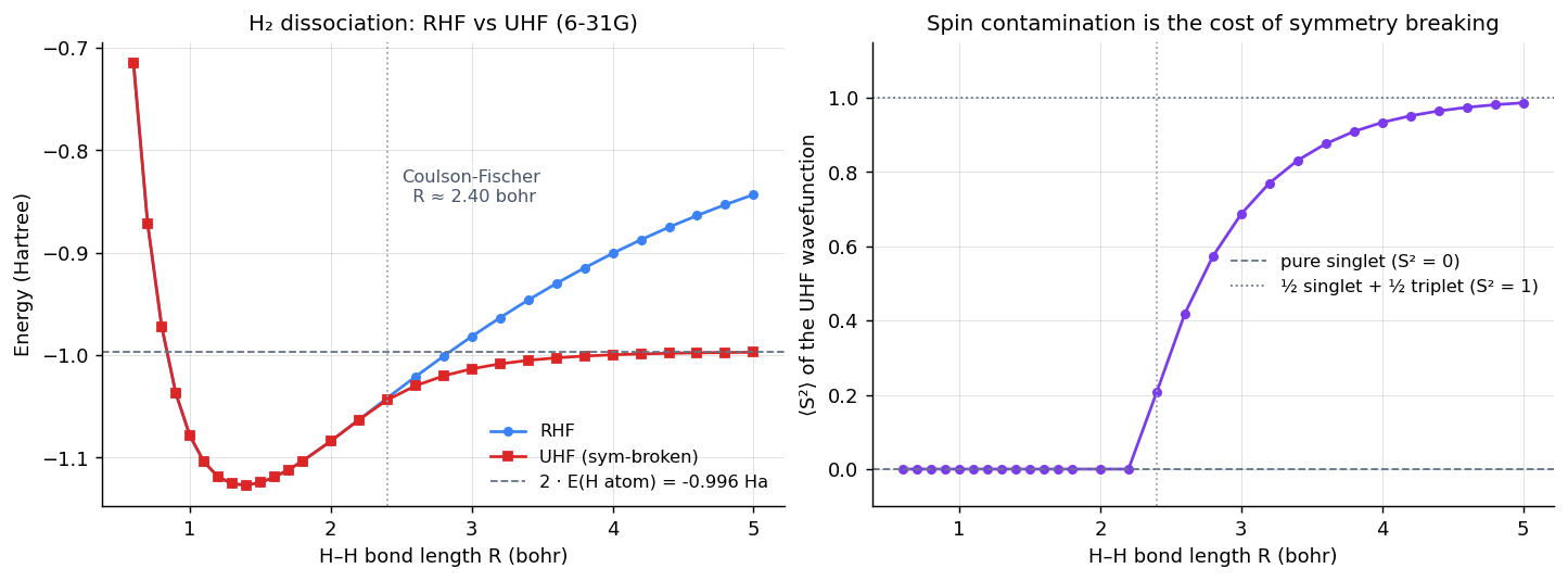
Three things to read off. (a) Below $R\approx 2.4$ bohr the RHF and UHF curves are identical to numerical precision — the constraint ${\psi }^{\alpha }={\psi }^{\beta }$ isn't doing any work, because the true ground state actually has that symmetry. (b) Past the Coulson-Fischer point the curves split. At $R=5$ bohr, RHF is wrong by 154 millihartrees (about 97 kcal/mol), while UHF is within 0.6 mHa of the exact dissociation limit $2\cdot E(\text{H})$. (c) The UHF wavefunction's $⟨S^2⟩$ rises from 0 toward 1 — UHF is no longer a pure singlet at large R; it's an equal mix of singlet and triplet (a singlet has $S^2=0$, triplet $S^2=2$, equal mix $S^2=1$). That's the famous "spin contamination" of UHF, and it's the price you pay for getting the right energy.

The clean version of the original question

The Fock operator gives you a basis of single-particle orbitals, full stop. The N electrons, and how they get spread across those orbitals, is a separate piece of the problem — a piece that lives in the ansatz, not in the Fock operator. The N/2 in RHF is the closed-shell-singlet choice, written explicitly into the wavefunction. UHF, ROHF, and GHF make different choices. The Coulson-Fischer split shows that this isn't a matter of taste: when the true ground state breaks the symmetry of the constrained ansatz, the constrained ansatz silently gives the wrong answer. The orbitals are derived; the way you fill them is modeling.

The code

Full self-contained PySCF script and a slimmed printout of the curve are below. The full sweep (and the figure-rendering code) is in my notes repo.

"""
H2 dissociation: RHF vs UHF in PySCF (6-31G basis).

UHF needs a deliberately spin-broken initial guess to find the
symmetry-broken solution past the Coulson-Fischer point.
We use the textbook HOMO-LUMO mixing trick:
  C_alpha[:, HOMO] =  cos(t) * C_RHF[:, HOMO] + sin(t) * C_RHF[:, LUMO]
  C_beta [:, HOMO] =  cos(t) * C_RHF[:, HOMO] - sin(t) * C_RHF[:, LUMO]
"""
import numpy as np
from pyscf import gto, scf

BASIS = "6-31g"

def uhf_broken(mol, mixing_angle=0.3):
    mf_r = scf.RHF(mol).run(verbose=0)
    C = mf_r.mo_coeff
    nocc = mol.nelectron // 2
    homo, lumo = nocc - 1, nocc
    Ca, Cb = C.copy(), C.copy()
    c, s = np.cos(mixing_angle), np.sin(mixing_angle)
    Ca[:, homo] =  c * C[:, homo] + s * C[:, lumo]
    Cb[:, homo] =  c * C[:, homo] - s * C[:, lumo]
    nao = mol.nao_nr()
    occ_a = np.zeros(nao); occ_a[:nocc] = 1
    occ_b = np.zeros(nao); occ_b[:nocc] = 1
    mf_u = scf.UHF(mol)
    dm0 = mf_u.make_rdm1((Ca, Cb), (occ_a, occ_b))
    mf_u.kernel(dm0=dm0)
    return mf_u

print(f"{'R (bohr)':>9} {'E_RHF':>11} {'E_UHF':>11} {'gap':>9} {'<S^2>':>9}")
for R in np.concatenate([np.linspace(0.6, 1.8, 7),
                         np.linspace(2.0, 5.0, 8)]):
    mol = gto.M(atom=f"H 0 0 0; H 0 0 {R}",
                basis=BASIS, unit="Bohr", verbose=0)
    e_rhf = scf.RHF(mol).run(verbose=0).e_tot
    mf_u = uhf_broken(mol)
    s2, _ = mf_u.spin_square()
    print(f"{R:9.2f} {e_rhf:11.5f} {mf_u.e_tot:11.5f} "
          f"{e_rhf - mf_u.e_tot:9.4f} {s2:9.4f}")

 R (bohr)       E_RHF       E_UHF       gap     <S^2>
     0.60    -0.71484    -0.71484   -0.0000   -0.0000
     0.80    -0.97204    -0.97204    0.0000    0.0000
     1.00    -1.07852    -1.07852    0.0000   -0.0000
     1.20    -1.11860    -1.11860    0.0000    0.0000
     1.40    -1.12674    -1.12674    0.0000    0.0000   ← R_eq
     1.60    -1.11894    -1.11894    0.0000    0.0000
     1.80    -1.10323    -1.10323   -0.0000    0.0000
     2.00    -1.08381    -1.08381   -0.0000    0.0000
     2.40    -1.04177    -1.04362    0.0018    0.2072   ← past CF point
     2.80    -1.00089    -1.02010    0.0192    0.5738
     3.20    -0.96342    -1.00840    0.0450    0.7702
     3.60    -0.92996    -1.00252    0.0726    0.8761
     4.20    -0.88731    -0.99868    0.1114    0.9512
     5.00    -0.84319    -0.99708    0.1539    0.9862

Reference:  2 · E(H atom, 6-31G) = -0.99647 Ha
Coulson-Fischer point:  R ≈ 2.4 bohr (1.27 angstrom)
Exact H2 (Kolos-Wolniewicz):  E = -1.17447 Ha at R_eq = 1.4 bohr

References

• Coulson, C. A. & Fischer, I. (1949). "Notes on the molecular orbital treatment of the hydrogen molecule." Philosophical Magazine, 40(303), 386–393. (The original paper on symmetry-broken HF and the bond-length point named after them.)
• Szabo, A. & Ostlund, N. S. (1996). Modern Quantum Chemistry, Dover. Chapter 3 (RHF) and Chapter 3.8 (UHF and spin contamination).
• Pople, J. A. & Nesbet, R. K. (1954). "Self-consistent orbitals for radicals." J. Chem. Phys., 22(3), 571–572. (The original UHF formulation.)
• Roothaan, C. C. J. (1960). "Self-consistent field theory for open shells of electronic systems." Rev. Mod. Phys., 32, 179–185. (The original ROHF formulation.)

Related on this site

The main Hartree-Fock page covers the Fock equations and SCF loop. Brute-force HF implements the loop from scratch. From scratch on H₂ derives the equations carefully. This page is the one that explains the part those pages tend to skip: where the electron count enters and what it actually constrains.