Brute-Force Hartree-Fock

Quantum Chemistry

A from-scratch Hartree-Fock framework written deliberately to be slow and visible rather than fast. The companion analytic-Gaussian Hartree-Fock page solves the integrals in closed form using the Gaussian product theorem; this page solves the same problem by gridding three-dimensional space and adding things up. The point is to see the math.

Bicycle, not motorcycle

Production quantum-chemistry codes are dense with optimizations: McMurchie-Davidson recursion for two-electron integrals, density fitting, J/K screening, integral-direct SCF, batched BLAS calls, OpenMP. Reading them is like looking at a motorcycle when you don't yet understand a bicycle. This code is the bicycle. Every step is its own object with one job. You can swap the basis (Slater for Gaussian), the Laplacian (3-point for 9-point), the integrator (cubic grid for Lebedev) without touching anything else.

Architecture

The core abstractions:

Atom, Molecule: Plain data: a charge plus a position; a list of atoms.
Slater1s: A normalized 1s Slater orbital $ϕ (r) = (ζ^{3} / π)^{1/2} e^{- ζ ∣ r - R ∣}$ . Exposes a single .value(r) method.
CubicGrid + GridIntegrator3D: Uniform cubic grid over $[- L, L]^{3}$ . Integration is just $\sum_{i} f (r_{i}) Δ V$ — no quadrature weights, no symmetry tricks, just rectangles.
NuclearPotential, NuclearRepulsionEnergy: The attractive electron-nucleus potential $- \sum_{A} Z_{A} /∣ r - R_{A} ∣$ and the classical nuclear-nuclear repulsion $\sum_{A < B} Z_{A} Z_{B} /∣ R_{A} - R_{B} ∣$ .
ThreePointLaplacianStencil3D: A 7-point central-difference Laplacian: $\nabla^{2} f \approx \frac{f ( x + h , y , z ) + f ( x - h , y , z ) + f ( x , y + h , z ) + f ( x , y - h , z ) + f ( x , y , z + h ) + f ( x , y , z - h ) - 6 f ( x , y , z )}{h ^{2}}$ The kinetic operator wraps this with a factor of $- 1/2$ .
KineticEnergyOperator, NuclearAttractionOperator, HamiltonianOperator: Each is a thin wrapper that knows how to .apply(wavefunction, r) to evaluate the operator's action on a wavefunction at a point. The Hamiltonian sums its terms.
MatrixElementBuilder: Given a basis and an integrator, computes $M_{ij} = ⟨ ϕ_{i} ∣ \hat{O} ∣ ϕ_{j} ⟩$ by integrating $ϕ_{i}^{*} (r) [\hat{O} ϕ_{j}] (r)$ over the grid.
solve_generalized_eigenproblem: Standard $S^{- 1/2}$ symmetric orthogonalization, then diagonalize, then transform back. Returns orbital energies and AO coefficients.

What it solves right now

H₂⁺: one electron, two protons. Only the one-electron Hamiltonian is needed — $\hat{H} = - \frac{1}{2} \nabla^{2} - \frac{1}{∣ r - R _{A} ∣} - \frac{1}{∣ r - R _{B} ∣}$ — and there is no electron-electron interaction yet, so this is not yet a true Hartree-Fock calculation. But the same machinery (basis, grid, operators, matrix builder, generalized eigenproblem) is what Hartree-Fock needs; the missing piece is the two-electron tensor and the SCF loop, sketched in Future Directions.

For each internuclear distance $R$ , the driver:

Builds the molecule and a two-element Slater basis (one orbital per nucleus).
Builds the overlap matrix $S_{ij}$ by gridding $ϕ_{i} ϕ_{j}$ .
Builds $H_{ij}$ by gridding $ϕ_{i} \hat{H} ϕ_{j}$ , where the kinetic term uses the finite-difference Laplacian.
Solves $H C = SCE$ via symmetric orthogonalization.
Adds the nuclear repulsion $1/ R$ .

The full code

import numpy as np
import matplotlib.pyplot as plt

# ============================================================
# Geometry
# ============================================================

class Atom:
    def __init__(self, charge, position):
        self.charge = float(charge)
        self.position = np.array(position, dtype=float)


class Molecule:
    def __init__(self, atoms):
        self.atoms = atoms


# ============================================================
# Basis functions
# ============================================================

class Slater1s:
    def __init__(self, zeta, R):
        self.zeta = zeta
        self.R = np.array(R)  # location of atom
        self.norm = (self.zeta**3 / np.pi)**0.5

    def value(self, r):
        distance = np.linalg.norm(r - self.R)
        return self.norm * np.exp(-1.0 * self.zeta * distance)

# ============================================================
# Integration utilities
# ============================================================

class CubicGrid:
    def __init__(self, length, pts_per_axis):
        self.length = length  # really only the half-length
        self.pts_per_axis = pts_per_axis
        self.x = np.linspace(-self.length, self.length, pts_per_axis)
        self.y = np.linspace(-self.length, self.length, pts_per_axis)
        self.z = np.linspace(-self.length, self.length, pts_per_axis)

        self.dx = self.x[1] - self.x[0]
        self.dy = self.y[1] - self.y[0]
        self.dz = self.z[1] - self.z[0]

        self.volume_element = self.dx * self.dy * self.dz

    def points(self):
        for x in self.x:
            for y in self.y:
                for z in self.z:
                    yield np.array([x, y, z], dtype=float)

class GridIntegrator3D:
    def __init__(self, grid):
        self.grid = grid

    def integrate(self, scalar_function):
        result = 0
        for pt in self.grid.points():
            result += scalar_function(pt) * self.grid.volume_element
        return result

# ============================================================
# Electron-nuclear attraction
# ============================================================

class NuclearPotential:
    def __init__(self, atoms):
        self.atoms = atoms

    def value(self, r):
        total = 0.0
        for atom in self.atoms:
            distance = np.linalg.norm(r - atom.position)
            distance = max(distance, 1e-8)
            total += -atom.charge / distance
        return total

# ============================================================
# Nuclear-nuclear repulsion
# ============================================================

class NuclearRepulsionEnergy:
    """
    Classical nuclear-nuclear repulsion:
        E_nn = sum_{A < B} Z_A Z_B / |R_A - R_B|
    """
    def __init__(self, atoms):
        self.atoms = atoms

    def value(self):
        total = 0.0
        for i, atom_i in enumerate(self.atoms):
            for j, atom_j in enumerate(self.atoms):
                if j <= i:
                    continue
                distance = np.linalg.norm(atom_i.position - atom_j.position)
                total += atom_i.charge * atom_j.charge / distance
        return total

# ============================================================
# Finite-difference Laplacian stencil
# ============================================================

class ThreePointLaplacianStencil3D:
    """
    Standard 7-point 3D Laplacian stencil applied to a scalar field f(r).
    """
    def __init__(self, h=1e-4):
        self.h = float(h)

    def apply(self, field, r):
        h = self.h
        x, y, z = r
        center = field.value(r)
        return (
            field.value(np.array([x + h, y, z]))
            + field.value(np.array([x - h, y, z]))
            + field.value(np.array([x, y + h, z]))
            + field.value(np.array([x, y - h, z]))
            + field.value(np.array([x, y, z + h]))
            + field.value(np.array([x, y, z - h]))
            - 6.0 * center
        ) / h**2

class LaplacianOperator:
    def __init__(self, stencil):
        self.stencil = stencil

    def apply(self, field, r):
        return self.stencil.apply(field, r)

# ============================================================
# Operators
# ============================================================
#
# operators are "applied" differently — in QM "apply" can mean different
# things, so this thin abstraction is just a wrapper around the actual
# mathematical operation.

class KineticEnergyOperator:
    """T = -1/2 nabla^2"""
    def __init__(self, laplacian):
        self.laplacian = laplacian

    def apply(self, wavefunction, r):
        return -0.5 * self.laplacian.apply(wavefunction, r)

class NuclearAttractionOperator:
    def __init__(self, potential):
        self.potential = potential

    def apply(self, wavefunction, r):
        return self.potential.value(r) * wavefunction.value(r)

class HamiltonianOperator:
    def __init__(self, terms):
        self.terms = terms

    def apply(self, wavefunction, r):
        return sum(term.apply(wavefunction, r) for term in self.terms)

class IdentityOperator:
    def apply(self, field, r):
        return field.value(r)

# ============================================================
# Matrix element builder
# ============================================================

class MatrixElementBuilder:
    def __init__(self, basis, integrator):
        self.basis = basis
        self.integrator = integrator

    def matrix_element(self, operator, bra, ket):
        def integrand(r):
            return bra.value(r) * operator.apply(ket, r)
        return self.integrator.integrate(integrand)

    def build_matrix(self, operator):
        n = len(self.basis)
        M = np.zeros((n, n))
        for i, bra in enumerate(self.basis):
            for j, ket in enumerate(self.basis):
                M[i, j] = self.matrix_element(operator, bra, ket)
        return M


# ============================================================
# Linear algebra
# ============================================================

def solve_generalized_eigenproblem(H, S):
    """Solve H c = S c eps via S^(-1/2) symmetric orthogonalization."""
    s_vals, s_vecs = np.linalg.eigh(S)
    S_inv_sqrt = s_vecs @ np.diag(1.0 / np.sqrt(s_vals)) @ s_vecs.T
    H_ortho = S_inv_sqrt.T @ H @ S_inv_sqrt
    energies, y = np.linalg.eigh(H_ortho)
    C = S_inv_sqrt @ y
    return energies, C

# ============================================================
# Driver
# ============================================================

def make_h2_plus(R):
    return Molecule([
        Atom(1.0, [0, 0, -R/2]),
        Atom(1.0, [0, 0,  R/2]),
    ])

def make_basis(molecule):
    return [Slater1s(1.0, atom.position) for atom in molecule.atoms]

def compute_energy(R):
    mol = make_h2_plus(R)
    basis = make_basis(mol)

    grid = CubicGrid(6.0, 30)            # half-length 6 Bohr, 30 points/axis
    integrator = GridIntegrator3D(grid)
    builder = MatrixElementBuilder(basis, integrator)

    potential = NuclearPotential(mol.atoms)
    nuclear_repulsion = NuclearRepulsionEnergy(mol.atoms)

    stencil = ThreePointLaplacianStencil3D(h=1e-4)
    laplacian = LaplacianOperator(stencil)

    kinetic = KineticEnergyOperator(laplacian)
    nuclear = NuclearAttractionOperator(potential)
    H_op = HamiltonianOperator([kinetic, nuclear])

    S = builder.build_matrix(IdentityOperator())
    H = builder.build_matrix(H_op)

    energies, _ = solve_generalized_eigenproblem(H, S)

    # H2+ has only one electron — take the lowest orbital.
    E_total = energies[0] + nuclear_repulsion.value()
    return E_total


def run_curve():
    Rs = np.linspace(0.5, 4.0, 20)
    Es = [compute_energy(R) for R in Rs]

    plt.plot(Rs, Es, marker='o')
    plt.xlabel("R (Bohr)")
    plt.ylabel("Total energy (Hartree)")
    plt.title("H2+ ground state — brute-force grid solver")
    plt.grid()
    plt.show()


if __name__ == "__main__":
    run_curve()

Result

Running run_curve() sweeps $R$ from 0.8 to 4.0 Bohr. The textbook H₂⁺ minimum sits at $R \approx 2.0$ Bohr with $E \approx - 0.6026$ Hartree. With the brute-force solver at 24 grid points per axis, the minimum instead lands near $R \approx 2.6$ Bohr at $E \approx - 0.56$ Hartree — bound (below the $- 1/2$ Hartree dissociation limit), and qualitatively right, but shifted by the discretization error of a 24³ uniform cubic grid. Increasing the grid count tightens both numbers; the cost is roughly cubic in the points-per-axis.

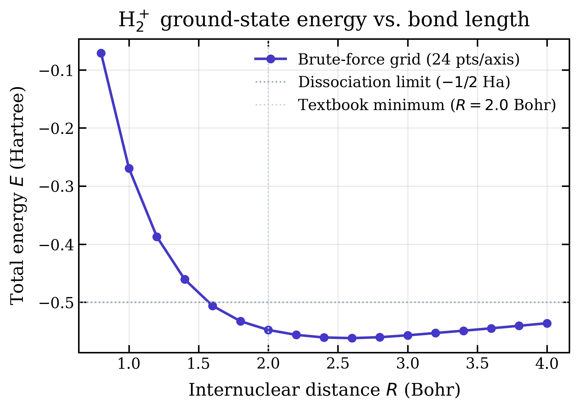
H2+ ground-state energy as a function of internuclear distance R, computed with a 24-point cubic grid. Curve is repulsive at small R, has a bound minimum near R=2.6 Bohr, and approaches -1/2 Ha (the dissociation limit) at large R.

The two interesting features of this curve:

The minimum sits below the $- 1/2$ -Hartree dotted line — that's an H atom + bare proton at infinity. Anything below that line is a bound molecule. The whole point of computing this curve is to demonstrate binding from first principles.
At large $R$ the curve relaxes back toward $- 1/2$ : the two nuclei stop sharing the electron, and you're left with a hydrogen atom plus an isolated proton, total energy $- 0.5$ Ha.

Why this is where the C++ port matters

The 24³-point grid above is the practical limit in pure Python: the curve takes about 25 seconds to generate, and the inner loop is a triply-nested Python for over grid points calling np.linalg.norm seven times per Laplacian application. The cost scales like $O (N^{3})$ in the points-per-axis. Doubling the resolution to 48³ is 8× more work — call it three to four minutes per curve — which is the boundary where casual exploration stops being casual.

More to the point: the qualitative error in the result above is visible. The minimum sits at $R \approx 2.6$ Bohr instead of $2.0$ , the well depth undershoots the literature $- 0.6026$ Ha by about $0.04$ Ha, and refining the grid is the only obvious way to fix it without changing the algorithm. A 48-point or 64-point grid would tighten both numbers; in Python, that's a coffee-and-come-back. In a compiled implementation with the same algorithm — same Slater basis, same finite-difference Laplacian, same cubic-grid integrator — the same problem at 64³ points should run in seconds rather than minutes. That's the concrete motivation for the C++ port: not a different theory, just enough headroom in the constant factor to make the grid resolution high enough that the result stops being qualitatively wrong.

Future Directions

What's not yet wired through. Each item is sketched somewhere in the project but not connected end-to-end.

Two-electron repulsion tensor

The four-index tensor $(μν ∣ λσ) = \iint ϕ_{μ} (r_{1}) ϕ_{ν} (r_{1}) \frac{1}{∣ r _{1} - r _{2} ∣} ϕ_{λ} (r_{2}) ϕ_{σ} (r_{2}) d r_{1} d r_{2}$ requires a six-dimensional integration. Brute force is unkind here: a 30-point cubic grid in 6D is $3 0^{6} \approx 7 \times 1 0^{8}$ points per integral, times 16 integrals for a two-basis-function H₂, times 1/r₁₂ singularity handling. The naive nested-loop sketch in the older hf.py works in principle but is impractical past trivial cases. The realistic path is a Becke- or Lebedev-style atom-centered grid and a Poisson solve for the potential, not direct 6D summation.

Coulomb and exchange operators

Once the two-electron tensor is available, the Fock matrix $F_{μν} = H_{μν}^{core} + \sum_{λσ} P_{λσ} [(μν ∣ λσ) - \frac{1}{2} (μ λ ∣ ν σ)]$ is just two tensor contractions with the density matrix. Both fit the operator/.apply() pattern already in place — they just need a .contract_with(P) method that returns a 2D matrix from the 4D tensor.

SCF loop

Once the Fock matrix can be assembled from a density, the SCF loop is the same as on the analytic-Gaussian page: diagonalize, build a new density, mix with damping, repeat until the density stops changing. The infrastructure here already does the diagonalization and density build for the one-electron case.

Slater-to-Gaussian basis fitting

The C++ implementation begins with a Levenberg-Marquardt fit of an STO-NG expansion (a Slater orbital approximated by N Gaussians). That gives the ergonomics of Slater orbitals (one parameter per atom) with the integrability of Gaussians (analytic two-electron integrals). Currently the C++ side has the matrix/vector primitives and a Blue-algorithm Euclidean norm in place; the LM fitter and the SCF driver are stubs.

C++ port

A parallel C++ implementation — same architecture, real types, no NumPy. Currently builds out the linear algebra primitives (Matrix<T>, VectorView<T>, enorm via Blue's algorithm) before the solver. The eventual goal is identical results to the Python version on the same problem, with timings that show what the abstraction is costing.

Why bother

Once you've watched H₂⁺ converge from a 7-point Laplacian and a cubic grid of integrands, the Gaussian-product magic on the analytic page stops feeling like magic. The integrals on that page compute the same numbers this page is computing, just in milliseconds instead of minutes. Both are useful. One teaches; the other ships.