“Know how to solve every problem that has been solved.” “What I cannot create, I do not understand.” — Richard Feynman

Project: Gamma Knife Dose Simulation

Projects

Two hundred weak beams, one hot point: the geometry of stereotactic radiosurgery, computed and validated. Stack: Python · NumPy · Monte Carlo attenuation check. A physics teaching model — not a treatment-planning tool.

What this is

A Gamma Knife treats a brain lesion without a scalpel by pointing roughly two hundred cobalt-60 beams at one point. Each beam on its own is too weak to destroy tissue — it deposits a long, gentle stripe of dose on its way through the head. But every beam passes through the same few cubic millimeters, and there the doses add. One beam burns a line; two hundred burn a point. This project builds the dose model from three pieces of freshman physics — exponential attenuation, inverse-square spreading, a collimated beam profile — and then quantifies exactly how the point wins over the lines. Lars Leksell proposed the idea in 1951 and treated the first patients with a prototype in the 1960s; the collimator sizes here (4, 8, 16 mm) are the real ones.

The model, and its edges

Each beam is a narrow cone of 1.25 MeV photons (the average of cobalt-60's 1.17 and 1.33 MeV lines) converging on the isocenter from a source 40 cm away. At a point $p$ inside a spherical water phantom of radius 8 cm, the primary dose from one beam is

D_{i} (p) = e^{- μ d_{i} (p)} (\frac{SAD}{r _{i} ( p )})^{2} exp (- \frac{b _{i} ( p ) ^{2}}{2 σ ^{2}}),

where $d_{i}$ is the tissue path length from skull entry, $r_{i}$ the distance from the source, $b_{i}$ the distance off the beam's central axis, and $σ$ is set by the collimator width (FWHM = 4, 8, or 16 mm). The attenuation coefficient is the NIST value for water at 1.25 MeV, $μ / ρ = 0.0632 c m^{2} /g$ . The total dose is the sum over beams whose axes are spread over a helmet-like spherical cap.

Stated plainly, this is a primary-photon model: it tracks the photons that arrive unscattered and ignores what happens after they interact. A full Monte Carlo transport calculation adds Compton-scattered dose, electron buildup at the surface, and bone/air heterogeneities — corrections a clinic cannot ignore and this page can, because the phenomenon being studied (dose concentration by convergence) lives entirely in the geometry.

MU = 0.0632          # 1/cm, water at 1.25 MeV (NIST mass attenuation x 1 g/cm^3)
R_HEAD = 8.0         # cm, spherical water phantom
SAD = 40.0           # cm, source-to-isocenter distance

def beam_dose(points, u, sigma):
    """Primary dose of one beam (axis through origin, direction u,
    source at SAD*u) at an array of points, shape (M, 3)."""
    s = SAD * u
    w = points - s                                   # source -> point
    r = np.linalg.norm(w, axis=1)
    v = w / r[:, None]
    # ray-sphere entry: |s + t v| = R_HEAD, smaller positive root
    b_ = np.einsum("j,ij->i", s, v)
    disc = b_**2 - (SAD**2 - R_HEAD**2)
    t_entry = -b_ - np.sqrt(np.maximum(disc, 0.0))
    depth = np.maximum(0.0, r - t_entry)             # path length in tissue
    # off-axis distance from the central axis (line through origin along u)
    proj = np.einsum("ij,j->i", points, u)
    b_axis = np.linalg.norm(points - proj[:, None] * u, axis=1)
    return np.exp(-MU * depth) * (SAD / r)**2 * np.exp(-b_axis**2 / (2 * sigma**2))

Validation before physics

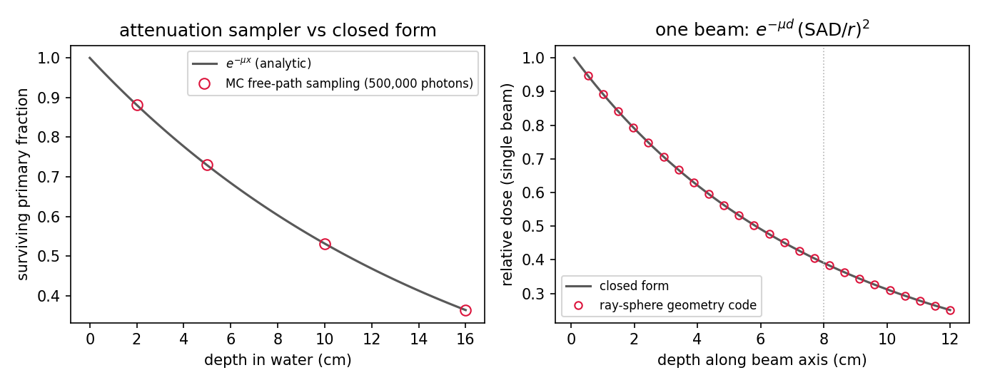
Two checks, both against closed forms. The vectorized ray-sphere geometry is compared with the hand-derived on-axis formula $e^{- μ (R - z)} (SAD / (SAD - z))^{2}$ — agreement to $4 \times 1 0^{- 16}$ , machine precision. And a small Monte Carlo samples 500,000 photon free paths from $ℓ = - ln ξ / μ$ and counts survivors past each depth; the survival fractions land on $e^{- μx}$ to 0.17%, which is the expected statistical noise. The attenuation model and its implementation are both doing what they claim.

[1] geometry vs closed form  max |err| = 4.44e-16
[2] MC survival vs exp(-mu x), 500,000 photons:
      x =  2.0 cm   MC 0.88206   analytic 0.88126
      x =  5.0 cm   MC 0.73033   analytic 0.72906
      x = 10.0 cm   MC 0.53163   analytic 0.53153
      x = 16.0 cm   MC 0.36395   analytic 0.36378
      max relative deviation = 0.17%

$Two panels. Left: surviving primary photon fraction versus depth in water, Monte Carlo points at 2, 5, 10, 16 cm lying on the analytic exponential curve. Right: single-beam relative dose versus depth along the beam axis, open circles from the ray-sphere geometry code lying exactly on the closed-form attenuation-times-inverse-square curve, dropping from 1 to about 0.25 over 12 cm.$

The picture that is the whole idea

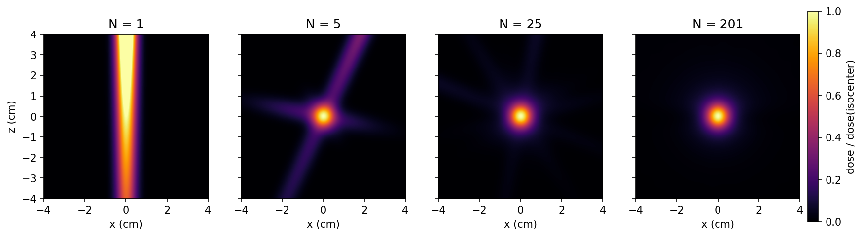
The same slice through the isocenter, computed with 1, 5, 25, and 201 beams, each map normalized to its own isocenter dose. With one beam the "treatment" is a corridor of full-strength dose straight through the head. Five beams make a star whose arms carry a fifth of the dose each. By 201, the arms have faded below 2% and what remains is a ball of dose the size of the collimator setting.

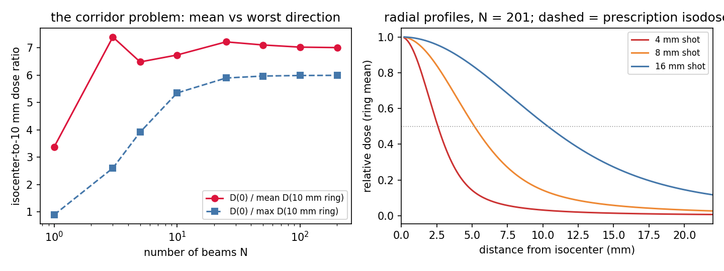
Four dose maps on a slice through the head phantom for N equals 1, 5, 25, and 201 beams, inferno colormap. N=1 shows a bright full-strength vertical corridor through the whole image. N=5 shows a five-armed star with a hot core. N=25 shows faint spokes around a bright central ball. N=201 shows only a compact bright ball at the center with no visible spokes.

The numbers underneath sharpen the story, and the first row contains the best fact on this page: with a single beam, the isocenter-to-worst-point ratio at 10 mm is 0.89 — less than one. The target is not even the hottest place on that ring. Upstream tissue sits closer to the source and behind less attenuating material, so a single beam always deposits more dose on the way in than at the lesion. Convergence doesn't just spare healthy tissue; it is the only way to make the target the maximum of the dose field at all.

[3] falloff vs number of beams (8 mm collimator):
      N     D0/mean(5mm)  D0/mean(10mm)  D0/max(10mm)
        1         1.60           3.38          0.89   <- target is NOT the hottest point
        3         2.02           7.40          2.60
        5         1.90           6.48          3.92
       10         1.89           6.74          5.35
       25         1.94           7.22          5.90
      201         1.92           7.01          5.99   <- worst direction 6x colder

[4] 50% isodose radius (N = 201) per collimator:
       4 mm shot:  r50 =  2.57 mm   penumbra 80->20% = 2.87 mm
       8 mm shot:  r50 =  5.18 mm   penumbra 80->20% = 5.86 mm
      16 mm shot:  r50 = 10.29 mm   penumbra 80->20% = 11.71 mm

[5] Co-60 after 5 years: 0.5181 of initial activity
    (3.5 Gy/min fresh -> 1.81 Gy/min; treatment times x1.93)

Two panels. Left: isocenter-to-10mm dose ratio versus number of beams on a log axis; the ring-mean ratio jumps from 3.4 at N=1 to about 7 and stays flat, while the ring-maximum ratio climbs from 0.89 at N=1 through 3.9 at N=5 to a plateau of 6 by N=25. Right: radial dose profiles for 4, 8, 16 mm collimators at N=201, sigmoid falloffs crossing the dashed 50% prescription line at 2.6, 5.2, and 10.3 mm respectively.

Note what the left panel says about diminishing returns: the mean falloff is already saturated by a handful of beams, but the worst-direction falloff — the number that decides whether some corridor of healthy tissue takes real dose — keeps improving until about 25 beams and only then plateaus near 6×. The extra 176 beams buy insurance in every direction at once, plus the freedom to block individual beams that would pass through something delicate.

Reading it like a treatment plan

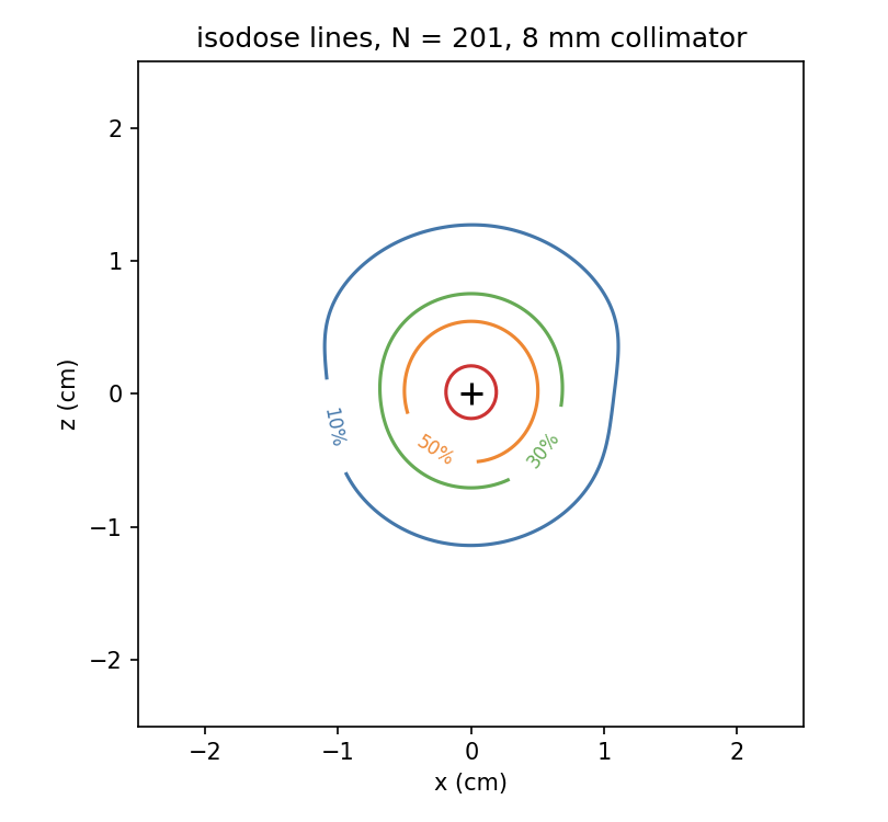
Isodose contour plot for 201 beams with an 8 mm collimator: nested closed contours at 90, 50, 30, and 10 percent of the isocenter dose around a central cross marker, roughly circular, slightly elongated vertically, with the 10 percent line at about 1.2 cm radius.

Clinical Gamma Knife plans are traditionally prescribed to the 50% isodose line — the surgeon draws the lesion, and the plan arranges for that surface to receive half the maximum dose. In this model the 50% radius comes out at 2.6, 5.2, and 10.3 mm for the 4, 8, and 16 mm collimators — the shot size tracks the collimator, as it should. The penumbra, the shell where dose falls from 80% to 20%, is 3 to 12 mm wide: that is the physics-imposed price of a Gaussian beam profile, and the reason radiosurgery targets are contoured in millimeters. The contours are slightly taller than they are wide — a real effect of the helmet geometry, since beams arrive from the upper hemisphere only and thin the dose along the polar axis less than the equatorial one.

One more piece of working arithmetic: cobalt-60 has a 5.27-year half-life, so after five years the sources hold $2^{- 5/5.27} = 0.518$ of their activity and every treatment takes 1.93× as long. That is the actual economics of these machines — the sources are swapped roughly every five to seven years not because they stop working but because treatment time doubles.

Try First

Each prompt asks a checkable question about the working code or math above — predict an output, derive a sign, state an invariant, find a bug. Commit to an answer before clicking "reveal." That commitment is the whole point: if your answer matched, you understand the piece you were looking at; if it didn't, that's the part worth re-reading.

predict

Before looking at the falloff table: with a single beam and the target at the center of the head, where is the maximum of the dose field?

why does this work

Each individual beam's depth profile is the same gentle exponential no matter how many beams there are. Why does adding beams sharpen the falloff around the target?

what if

The lesion sits 1 cm under the skull instead of at the center. What breaks in the symmetric-helmet plan, and what would you change?

Extensions

The model is deliberately minimal; every one of its omissions is a project.

Compton scatter by Monte Carlo. The free-path sampler is already validated; add Klein–Nishina sampling of the scattering angle and energy, transport the scattered photon, and measure how much dose the primary-only model misplaces — the classic buildup region near the surface should appear on its own.
Beam-weight optimization. For an off-center target, choose per-beam weights minimizing dose at specified organ-at-risk points subject to full dose at the target — a small constrained least-squares problem, solvable with gradient descent or as a quadratic program.
Shot packing. Real lesions are not spheres. Cover an irregular 3D target with multiple isocenters of different collimator sizes and score the plan with the clinical conformity indices (RTOG, Paddick).
A skull, not a water ball. Add a 6 mm bone shell ( $μ$ about 1.9× water's at this energy) and an air-filled sinus, and watch the isodose lines dent.
The proton comparison. Photons attenuate exponentially; protons stop at a depth and deposit most of their energy in the last few millimeters (the Bragg peak). Build the same figures for a scanned proton beam and compare the two ways physics offers to concentrate dose.

Everything above is generated by scripts/projects/gamma_knife.py — the figures, the falloff table, and the validation numbers come from one run of the model, not from a textbook screenshot.