Logistic Regression from Scratch

Machine Learning

Linear regression predicts a real number. Logistic regression predicts a probability. The data is the same shape — features in, target out — but the target is now a class label $y \in {0, 1}$ rather than a continuous value, and what you actually want from the model is $P (y = 1 ∣ x)$ . Linear regression cannot give you that directly: it predicts $x^{⊤} β$ which can run off to $\pm \infty$ , so calling its output a probability gives you values like $- 0.3$ or $1.4$ . Logistic regression is the smallest possible fix.

The fix: squash the linear output into (0, 1)

Take the linear combination $z = x^{⊤} β$ and pass it through a function that compresses $R$ into $(0, 1)$ . The sigmoid (or logistic) function is the standard choice:

σ (z) = \frac{1}{1 + e ^{- z}}

$σ$ is monotone increasing, $σ (- \infty) = 0$ , $σ (0) = 1/2$ , $σ (+ \infty) = 1$ . Its derivative is unusually clean: $σ^{'} (z) = σ (z) (1 - σ (z))$ . This is the function that turns the linear score $x^{⊤} β$ into a probability:

P (y = 1 ∣ x) = σ (x^{⊤} β)

The model has the same parameter $β$ as linear regression and the same design matrix $X$ with an intercept column. The only structural difference is the squash on the output. Why this choice rather than something else? Two reasons. First, $σ$ is the inverse of the log-odds: writing the model as $lo g \frac{P ( y = 1 )}{P ( y = 0 )} = x^{⊤} β$ says we're modelling the log-odds as a linear function of the features. Each coefficient $β_{j}$ tells you how much the log-odds change per unit of $x_{j}$ — that interpretability is why epidemiologists and credit-risk modelers actually use this rather than just "any squash function." Second, the loss derived from $σ$ is convex (no spurious local minima), and its gradient comes out to a remarkably clean form. Both fall out of the next step.

The loss: cross-entropy from maximum likelihood

For binary classification, the data are independent Bernoulli draws. The likelihood of observing $(x_{i}, y_{i})$ under the model is

P (y_{i} ∣ x_{i}, β) = σ (x_{i}^{⊤} β)^{y_{i}} (1 - σ (x_{i}^{⊤} β))^{1 - y_{i}}

— probability $σ (x^{⊤} β)$ when the label is 1, probability $1 - σ (x^{⊤} β)$ when it's 0. Taking the log, averaging across the dataset, and flipping the sign gives the loss we minimize:

L (β) = - \frac{1}{n} i = 1 \sum n [y_{i} lo g σ (x_{i}^{⊤} β) + (1 - y_{i}) lo g (1 - σ (x_{i}^{⊤} β))]

This is the cross-entropy loss (or equivalently the log-loss). It's the negative log-likelihood of the Bernoulli model, exactly parallel to how squared error is the negative log-likelihood of a Gaussian model in linear regression. Squared error assumes Gaussian noise; cross-entropy assumes Bernoulli noise — appropriate for 1 outcomes.

The gradient comes out beautifully. Using $σ^{'} (z) = σ (z) (1 - σ (z))$ and a few lines of algebra:

\nabla L (β) = \frac{1}{n} X^{⊤} (σ (Xβ) - y)

Compare with linear regression's gradient $\nabla L (β) = \frac{2}{n} X^{⊤} (Xβ - y)$ . The structure is identical — $X^{⊤} (prediction - target)$ — with the linear prediction $Xβ$ replaced by its sigmoid $σ (Xβ)$ . This pattern reappears in essentially every loss function used in deep learning, because the chain rule shapes the gradient that way whenever the loss is a clean function of the model output.

No closed form, so we descend

Setting $\nabla L = 0$ gives $X^{⊤} (σ (Xβ) - y) = 0$ , which is a system of nonlinear equations in $β$ . No closed form. This is where the closed-form-vs-iterative split between linear and logistic regression becomes real: we run gradient descent on $L (β)$ and stop when the gradient is small. The loss is convex (the Hessian is $\frac{1}{n} X^{⊤} diag (σ (Xβ) (1 - σ (Xβ))) X$ , which is positive semi-definite), so GD converges to the unique optimum — no local-minimum traps, no need for random restarts.

For Newton-style optimizers there's a specialized variant called iteratively reweighted least squares (IRLS) that converges in 10–20 iterations rather than thousands, and is the default in most statistics packages. For ML at scale, plain gradient descent (or stochastic gradient descent) wins because IRLS needs to factor the Hessian at every step.

The code

"""
Logistic regression from scratch.

Binary classification on two 2D Gaussian blobs. Fit by gradient descent
on the negative log-likelihood (a.k.a. cross-entropy loss). Report
accuracy, confusion matrix, and AUC.
"""

import numpy as np
import matplotlib.pyplot as plt


def sigmoid(z):
    """Numerically stable σ(z) = 1 / (1 + e^{-z})."""
    return np.where(z >= 0,
                    1.0 / (1.0 + np.exp(-z)),
                    np.exp(z) / (1.0 + np.exp(z)))


def cross_entropy(beta, X, y):
    """Average negative log-likelihood, computed without overflow.

    log(1 + e^z) = max(z, 0) + log(1 + e^{-|z|})    (softplus identity).
    """
    z = X @ beta
    return np.mean(np.maximum(z, 0.0) - z * y + np.log1p(np.exp(-np.abs(z))))


def cross_entropy_grad(beta, X, y):
    """∇ℒ(β) = (1/n) Xᵀ (σ(Xβ) − y).

    Same shape as linear regression's gradient — Xᵀ(prediction − target)
    — with the linear prediction replaced by σ applied to it.
    """
    p = sigmoid(X @ beta)
    return X.T @ (p - y) / len(y)


def gradient_descent(grad_f, x0, lr, n_iter, tol=1e-9):
    x = np.asarray(x0, dtype=float).copy()
    hist = [x.copy()]
    for _ in range(n_iter):
        g = grad_f(x)
        x = x - lr * g
        hist.append(x.copy())
        if np.linalg.norm(g) < tol:
            break
    return x, np.array(hist)


# Synthetic data: two 2D Gaussian blobs with shared covariance.
rng = np.random.default_rng(7)
n_per_class = 120
mu0 = np.array([-1.2, -1.2])
mu1 = np.array([+1.2, +1.2])
cov = np.array([[1.0, 0.3],
                [0.3, 1.0]])

X0 = rng.multivariate_normal(mu0, cov, n_per_class)
X1 = rng.multivariate_normal(mu1, cov, n_per_class)
X_raw = np.vstack([X0, X1])
y     = np.concatenate([np.zeros(n_per_class), np.ones(n_per_class)])
n     = len(y)

X = np.column_stack([np.ones(n), X_raw])  # design matrix with intercept


# Fit by gradient descent on cross-entropy.
beta_hat, hist = gradient_descent(
    lambda b: cross_entropy_grad(b, X, y),
    x0=np.zeros(3), lr=0.5, n_iter=1500
)


# Diagnostics
p_hat   = sigmoid(X @ beta_hat)
y_pred  = (p_hat >= 0.5).astype(int)
acc     = np.mean(y_pred == y)

# Confusion matrix
cm = np.zeros((2, 2), dtype=int)
for t, p in zip(y.astype(int), y_pred):
    cm[t, p] += 1

# AUC via trapezoidal integration of the ROC curve.
order  = np.argsort(-p_hat)
y_sort = y[order]
n_pos, n_neg = y_sort.sum(), (1 - y_sort).sum()
tpr = np.concatenate([[0.0], np.cumsum(y_sort)       / n_pos])
fpr = np.concatenate([[0.0], np.cumsum(1 - y_sort)   / n_neg])
auc = np.sum((fpr[1:] - fpr[:-1]) * 0.5 * (tpr[1:] + tpr[:-1]))


print("Logistic regression — two 2D Gaussian blobs")
print("-" * 60)
print(f"  fit β (intercept, β_x1, β_x2)  : "
      f"({beta_hat[0]:+.4f}, {beta_hat[1]:+.4f}, {beta_hat[2]:+.4f})")
print(f"  decision boundary slope        : {-beta_hat[1] / beta_hat[2]:+.4f}")
print(f"  final cross-entropy            : {cross_entropy(beta_hat, X, y):.4f}")
print(f"  accuracy                       : {acc:.4f}")
print(f"  AUC                            : {auc:.4f}")
print()
print("  Confusion matrix:")
print(f"            pred 0   pred 1")
print(f"   true 0    {cm[0,0]:4d}     {cm[0,1]:4d}")
print(f"   true 1    {cm[1,0]:4d}     {cm[1,1]:4d}")

Running it

Logistic regression — two 2D Gaussian blobs
------------------------------------------------------------
  fit β (intercept, β_x1, β_x2)  : (-0.2322, +1.8421, +2.3219)
  decision boundary slope        : -0.7934
  final cross-entropy            : 0.1539
  accuracy                       : 0.9375
  AUC                            : 0.9861

  Confusion matrix:
            pred 0   pred 1
   true 0     113        7
   true 1       8      112

What you can read off

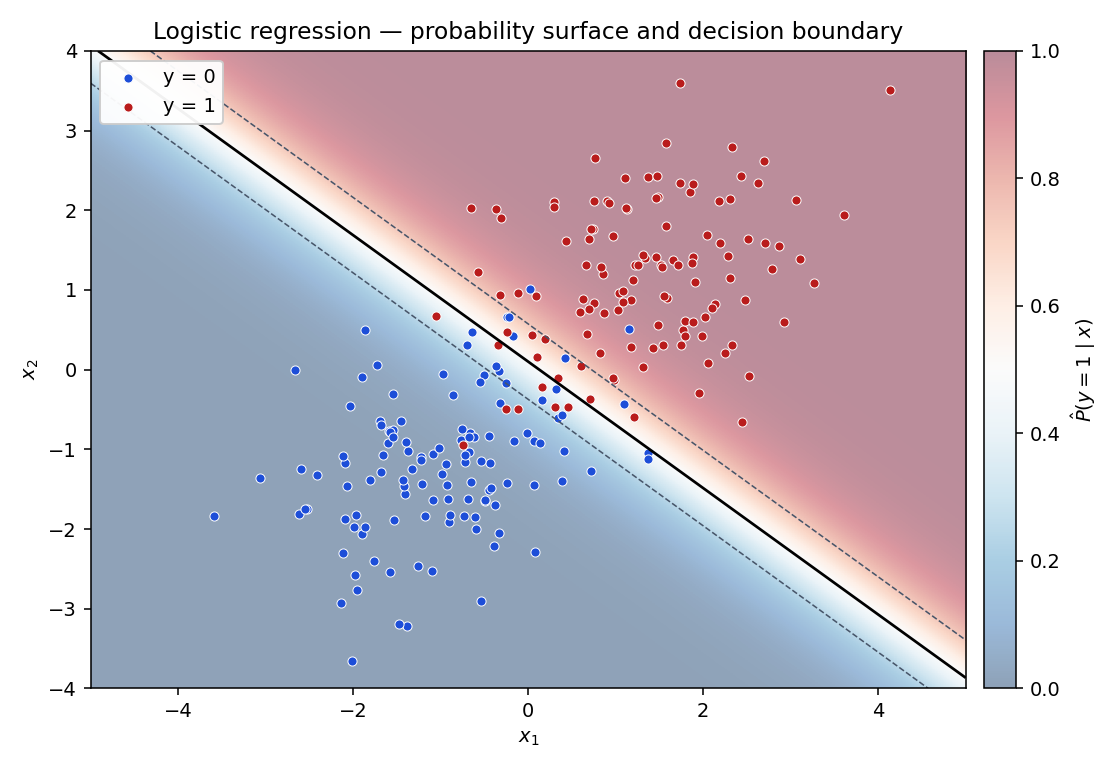
2D scatter plot of two Gaussian blobs (blue y=0, red y=1) overlaid on the smooth sigmoid probability surface. A diagonal solid line marks the 0.5 decision boundary; dashed lines mark the 0.25 and 0.75 contours. The blobs are well-separated with a few overlapping points near the boundary.

The decision boundary is linear. The set of points where $σ (x^{⊤} β) = 1/2$ is the same set where $x^{⊤} β = 0$ — a hyperplane. Logistic regression's "logistic" part is in how it scores points, not how it carves up space. The probability gradient is steepest along the normal to the boundary and asymptotes to 0 or 1 far away. Same boundary as a linear SVM, same boundary as Fisher's linear discriminant — what differs is the loss being optimized and what comes out for each point (a probability, a hinge score, a discriminant).

The coefficients say what matters. The fit found $β = (- 0.23, + 1.84, + 2.32)$ . The two non-intercept coefficients are similar in magnitude, which says $x_{1}$ and $x_{2}$ contribute roughly equally to the decision — matching the data, where the class centers are separated equally along both axes. The decision-boundary slope $- β_{1} / β_{2} \approx - 0.79$ tilts the boundary roughly along the orthogonal complement of $(β_{1}, β_{2})$ .

Standard diagnostics. Accuracy 93.75% and AUC 0.986 are both high, consistent with well-separated blobs. The confusion matrix shows 7 false positives and 8 false negatives out of 240 — the misclassifications are the points near the boundary you can see overlapping in the figure. Accuracy alone is a thin metric (a dataset with 99% class-0 has 99% accuracy from the constant prediction); AUC measures how well the model ranks positives above negatives across all thresholds, and is far more informative when classes are imbalanced.

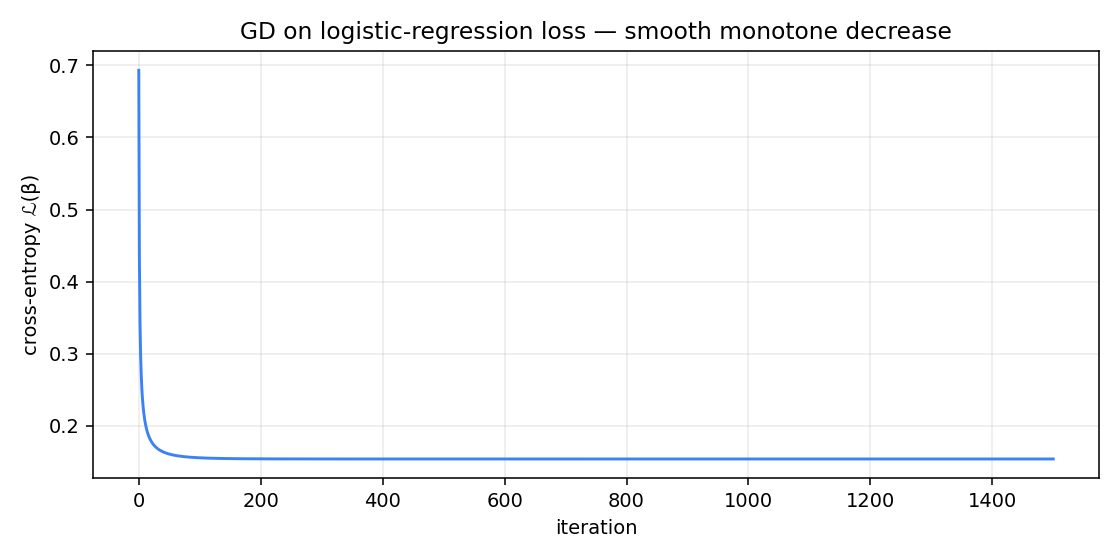
Cross-entropy loss as a function of gradient descent iteration. Starts at 0.69 (log 2, the random-guess baseline), drops sharply over the first 100 iterations, plateaus near 0.15 by iteration 200, slow asymptotic decrease afterward.

The loss starts at $lo g 2 \approx 0.693$ — the cross-entropy of the all-zeros initial $β$ , which predicts $σ (0) = 1/2$ for every point. That's the random-guess baseline. The fit drops to $\approx 0.15$ within a couple hundred iterations and crawls asymptotically toward an irreducible floor set by the genuine overlap between the two blobs. You will never push cross-entropy to zero on data that actually has class overlap, and that's correct — perfect zero would mean the model is overconfident about ambiguous points.

Why this matters beyond two-class problems

Logistic regression generalizes to multi-class problems by replacing the sigmoid with the softmax:

P (y = k ∣ x) = \frac{e ^{x^{⊤} β_{k}}}{\sum _{j = 1}^{K} e ^{x^{⊤} β_{j}}}

— one weight vector $β_{k}$ per class, the exponent normalizes them into a distribution over classes. The loss generalizes to multi-class cross-entropy, the gradient still has the form $X^{⊤} (\overset{p}{^} - y_{one-hot})$ , and the fit is again convex. This is "multinomial logistic regression" in statistics, "softmax classification" in ML — same algorithm, different name per audience.

More importantly, logistic regression is the simplest possible neural network. It's a single-layer linear function followed by a sigmoid (or softmax) activation. The whole machinery of deep learning — stacked layers, nonlinear activations between them, gradients via the chain rule — is what you get when you replace the single linear-plus-sigmoid step with many of them in sequence. Logistic regression is where the cross-entropy loss, the sigmoid activation, and the $X^{⊤} (σ (Xβ) - y)$ gradient structure all first appear. Every modern classifier is a fancier logistic regression at the output layer.

What this doesn't do

It can only learn linear boundaries. Two interlocking spirals, XOR data, anything not linearly separable — logistic regression fails because no hyperplane separates the classes. Standard fix: hand-engineer nonlinear features (add $x_{1} x_{2}$ , $x_{1}^{2}$ , $sin x_{1}$ ) into the design matrix, or learn them with a hidden layer (an MLP).

Probabilities are calibrated only if the linearity assumption holds. If the true log-odds are nonlinear in $x$ , logistic regression's probability outputs can be systematically wrong even when its decisions at threshold 0.5 are right. For high-stakes use (medical risk, credit scoring), you want to check calibration explicitly — plot predicted probability vs actual frequency, look for systematic deviation from the diagonal.

Separable data makes $∥ β ∥$ blow up. If two classes are perfectly separable, the MLE pushes $β$ to infinity along the separating direction — the cross-entropy keeps improving as the sigmoid sharpens toward a step function. In practice, you regularize: $L_{2}$ ridge penalty $+ λ ∥ β ∥^{2}$ or $L_{1}$ lasso. Or just stop the gradient descent early.

Class imbalance. If one class is 1% of the data, the model can hit 99% accuracy by predicting the majority class. The cross-entropy loss also gets dominated by the majority class. Standard remedies: weight the minority class higher in the loss, oversample/undersample, or evaluate with precision/recall/AUC rather than accuracy.

Where this shows up on the site

The output layer of every classification neural network on the site is a logistic regression (sigmoid for binary, softmax for multi-class) on top of learned features. The gradient descent page powers the fit. Maximum-likelihood derivations of regression losses are a recurring pattern in Bayesian inference — squared loss for Gaussian likelihoods, cross-entropy for Bernoulli, Poisson loss for count data, all variations on the same MLE recipe applied to different noise models. Logistic regression is the bridge from linear regression to neural networks; the next page picks up from here with multi-layer perceptrons.

Core idea

Logistic regression squashes a linear score through a sigmoid to get a probability, fits by maximum likelihood on the Bernoulli model, and gives you a linear decision boundary plus a smooth probability surface. The gradient is $X^{⊤} (σ (Xβ) - y) / n$ , the loss is convex, and gradient descent finds the unique optimum. Every classifier in deep learning has a logistic regression at its output.

Exercises

A full exercise set is available for this topic, structured as one worked example + 7 practice problems (across 7 surface contexts) + 2 pattern-resistant check problems.

Open the Logistic Regression exercise set → Recognize a problem as binary classification, model P(y=1|x) = σ(xᵀβ), fit by minimizing cross-entropy via gradient descent, then read decision boundary, probability calibration, and odds-ratio interpretation off the learned β.

References

Cox, D. R. (1958). The regression analysis of binary sequences. J. R. Stat. Soc. B, 20, 215. The original logistic regression paper.
Hastie, T., Tibshirani, R., & Friedman, J. (2009). The Elements of Statistical Learning, 2nd ed. Springer. Chapter 4 covers logistic regression in the same notation used here, plus IRLS and the multi-class extension.
Bishop, C. M. (2006). Pattern Recognition and Machine Learning. Springer. Chapter 4.3 is the cleanest treatment of logistic regression as a probabilistic classifier; Chapter 5 picks up where this page leaves off with neural networks.
McCullagh, P., & Nelder, J. A. (1989). Generalized Linear Models, 2nd ed. Chapman & Hall. The unifying framework where logistic regression is the binomial-family GLM.