Slater orbitals: the right shape, the wrong integrals

A Slater-type orbital is the physically correct shape. It has a cusp at the nucleus and an exponential tail — exactly what an electron's wavefunction does, because it is the hydrogenic solution. So a natural question: if Slater orbitals are right, why does almost every production code use Gaussians, which have neither the cusp nor the tail? The answer is not physics. It is integrals. See Slater orbitals for the shape itself; this page is about why that shape is so hard to compute with, and the handful of ways people get around it.

The difficulty: multicenter integrals

A molecular calculation needs integrals of products of basis functions sitting on different atoms. For Slater orbitals the difficulty grows sharply with how many centers are involved: one-center integrals are analytic, two-center integrals (overlap, kinetic, nuclear attraction) are hard but doable in elliptic coordinates, and the three- and four-center two-electron repulsion integrals are the wall — they have no general closed form at all.

The root cause is that Slater orbitals have no product theorem. The product of two Gaussians on different centers is a single Gaussian on a third center, which collapses every multicenter integral back to a one-center problem (see the Gaussian product theorem). The product of two Slater orbitals is not a Slater orbital on any center. Watch the difference directly:

import numpy as np
x = np.linspace(-5, 5, 2001)
A, B = -1.5, 1.5                      # two atomic centers

# Gaussians: the product of two collapses to ONE Gaussian at the midpoint
gA, gB = np.exp(-(x-A)**2), np.exp(-(x-B)**2)
P, K = (A+B)/2, np.exp(-(A-B)**2 / 2)
single = K * np.exp(-2*(x-P)**2)
print("Gaussian product == single Gaussian?  max err =", np.max(np.abs(gA*gB - single)))

# Slaters: the product has no single-center form
sA, sB = np.exp(-np.abs(x-A)), np.exp(-np.abs(x-B))
mid = (x > A) & (x < B)
print("Slater -ln(product) between centers is flat?  range =",
      np.ptp((-np.log(sA*sB))[mid]), " (= |A-B| =", abs(A-B), ")")

Gaussian product == single Gaussian?  max err = 5.2e-18
Slater -ln(product) between centers is flat?  range = 0.0  (= |A-B| = 3.0)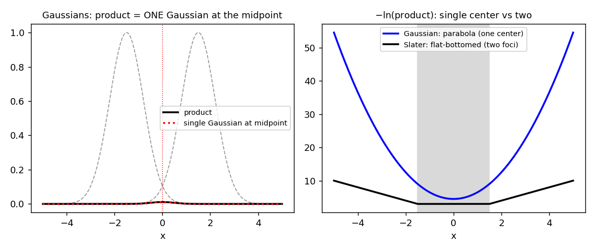

The reason is the difference between squared and linear distance. A Gaussian carries $|\vec{r}-\vec{A}{|}^2$, and $|\vec{r}-\vec{A}{|}^2+|\vec{r}-\vec{B}{|}^2$ completes the square into a single squared distance from the midpoint — that is the parallel-axis theorem, and it is why the product recenters. A Slater orbital carries the linear distance $|\vec{r}-\vec{A}|$, and the locus $|\vec{r}-\vec{A}|+|\vec{r}-\vec{B}|=\text{const}$ is an ellipse with two foci, not a sphere around one point. There is no center to collapse onto. Replacing the exponential with a rational does not help — the obstruction is the two-center geometry, not the transcendental function (see the Padé-STO negative result).

How to resolve it

1. Fit Gaussians to the Slater (STO-nG)

The dominant fix is to give up on Slater integrals entirely and approximate each Slater orbital by a fixed linear combination of $n$ Gaussians, least-squares fit to the Slater shape. You inherit the Gaussian product theorem and all of its analytic integral machinery (Obara-Saika, McMurchie-Davidson); you pay for it in the cusp and the tail, which a sum of Gaussians can only approximate. More Gaussians buy back accuracy. See STO-nG fitting for the fit itself.

2. Integrate numerically: the ADF way

Slater orbitals are not abandoned — ADF (Amsterdam Density Functional) is a production code built entirely on them, and it wins by refusing to do the integrals analytically at all. Because ADF is a density-functional code, it already needs numerical quadrature for the exchange-correlation energy, so it evaluates everything on atom-centered grids (historically the te Velde-Baerends Voronoi scheme, now Becke-style fuzzy-cell grids: a radial mesh times Lebedev angular points on each atom). The multicenter wall only exists if you insist on closed forms; on a grid it disappears. The Coulomb (Hartree) potential is handled by density fitting — fit the electron density in an auxiliary Slater set, then solve Poisson's equation — which sidesteps the four-center two-electron integrals.

Once the integrals are numerical, the Slater shape pays off: the correct cusp and tail mean fewer functions for the same accuracy, and the orbitals are excellent for relativistic all-electron work, heavy elements, and core properties (NMR, EPR). That is ADF's niche. The catch is exact Hartree-Fock exchange, whose four-center structure is expensive to do on a grid — which is why Gaussian codes still own Hartree-Fock and the post-Hartree-Fock methods.

3. Other routes

For diatomics, two-center integrals are analytic in elliptic (prolate spheroidal) coordinates. More generally, one can expand a Slater orbital on a distant center (Barnett-Coulson / Löwdin alpha-function expansions) or route the Coulomb interaction through an integral transform — the same Gaussian-and-Yukawa representations of $1/r_{12}$ that make the repulsion integral tractable (see representations of the Coulomb operator).

The verdict: Gaussians won the mainstream because the product theorem makes their integrals cheap and analytic, and you simply use more of them to fix the shape. Slater orbitals survive where their shape is worth the cost and a numerical-integration framework already exists — which, thanks to DFT and ADF, is a real and used corner of quantum chemistry, not a historical footnote.

Related on this site

• Slater orbitals — the shape itself: cusp, tail, the exponent ζ.
• Gaussian product theorem — why Gaussians collapse to one center (the parallel-axis theorem).
• Padé-STO negative result — why pulling the distance out of the exponential doesn't escape the multicenter problem.
• STO-nG fitting — the Gaussian-fit resolution in detail.
• Obara-Saika and McMurchie-Davidson — the Gaussian integral recurrences you inherit.
• Representations of the Coulomb operator — integral transforms of 1/r₁₂.