Harmonic Oscillator (Finite Difference)

Quantum Chemistry

The quantum harmonic oscillator is one of the most important problems in quantum mechanics. This page demonstrates solving the time-independent Schrödinger equation for the harmonic oscillator using the finite difference method.

Time-Independent Schrödinger Equation

The time-independent Schrödinger equation is:

- \frac{ℏ ^{2}}{2 m} \frac{d ^{2} ψ}{d x ^{2}} + V (x) ψ = E ψ

For the harmonic oscillator, the potential is:

V (x) = \frac{1}{2} m ω^{2} x^{2}

In atomic units ( $ℏ = m = 1$ ), this simplifies to:

- \frac{1}{2} \frac{d ^{2} ψ}{d x ^{2}} + \frac{1}{2} ω^{2} x^{2} ψ = E ψ

For $ω = 1$ , the potential becomes $V (x) = \frac{1}{2} x^{2}$ .

Finite Difference Discretization

We discretize the domain $x \in [x_{m i n}, x_{m a x}]$ into $N$ equally spaced points with spacing $Δ x$ . The second derivative is approximated using central differences:

\frac{d ^{2} ψ}{d x ^{2}} \approx \frac{ψ _{i + 1} - 2 ψ _{i} + ψ _{i - 1}}{( Δ x ) ^{2}}

This gives us a finite difference matrix:

D_{2} = \frac{1}{( Δ x ) ^{2}} - 2 10 ⋮ 1 - 2 1 ⋮ 01 - 2 ⋮ \dots \dots \dots ⋱

Hamiltonian Matrix

The Hamiltonian matrix is constructed as:

H = - \frac{1}{2} D_{2} + V

where $V$ is a diagonal matrix with elements $V_{ii} = \frac{1}{2} x_{i}^{2}$ . The eigenvalue problem becomes:

H ψ = E ψ

This is a standard eigenvalue problem that can be solved using standard linear algebra routines.

Analytical Solution

The analytical eigenvalues for the harmonic oscillator are:

E_{n} = ℏ ω (n + \frac{1}{2}), n = 0, 1, 2, \dots

In atomic units with $ω = 1$ :

E_{n} = n + \frac{1}{2}

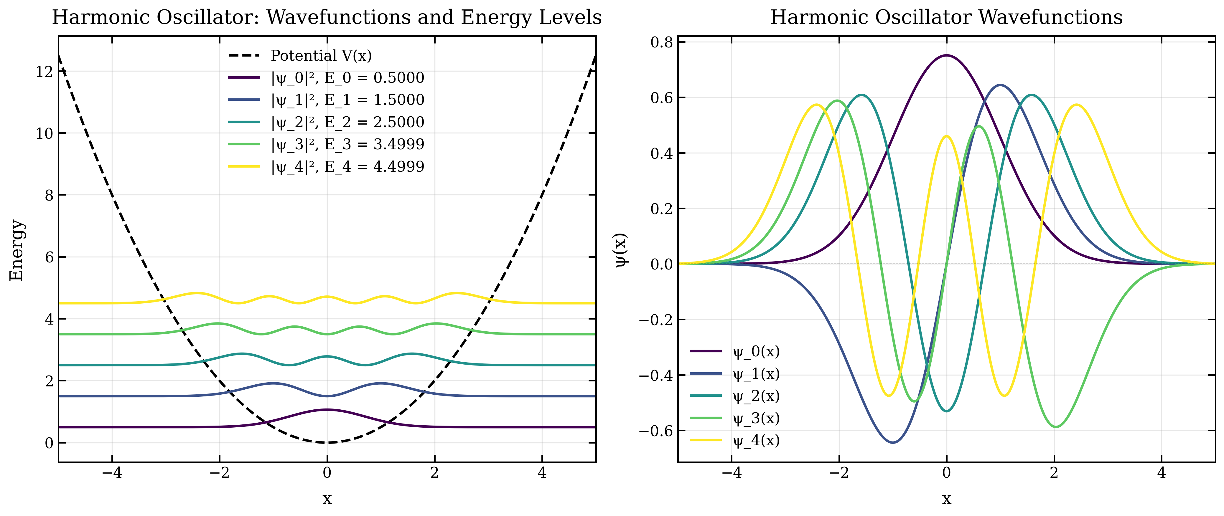
The ground state energy is $E_{0} = \frac{1}{2}$ , first excited state is $E_{1} = \frac{3}{2}$ , etc.

Python Implementation

The following code solves the harmonic oscillator using finite differences:

import numpy as np
import matplotlib.pyplot as plt
import matplotlib as mpl
from scipy.linalg import eigh

def set_publication_style():
    """Set publication-quality matplotlib style."""
    mpl.rcParams.update({
        'font.family': 'serif',
        'font.size': 12,
        'axes.labelsize': 14,
        'axes.titlesize': 16,
        'axes.linewidth': 1.2,
        'axes.labelpad': 8,
        'axes.titlepad': 10,
        'xtick.labelsize': 12,
        'ytick.labelsize': 12,
        'xtick.direction': 'in',
        'ytick.direction': 'in',
        'xtick.top': True,
        'ytick.right': True,
        'xtick.major.size': 6,
        'ytick.major.size': 6,
        'xtick.major.width': 1.2,
        'ytick.major.width': 1.2,
        'legend.fontsize': 12,
        'legend.frameon': False,
        'lines.linewidth': 2,
        'lines.markersize': 6,
        'figure.dpi': 100,
        'savefig.dpi': 300,
        'savefig.bbox': 'tight'
    })

set_publication_style()

# Parameters
N = 1000  # Number of grid points
x_min, x_max = -5.0, 5.0  # Domain boundaries
x = np.linspace(x_min, x_max, N)
dx = x[1] - x[0]  # Grid spacing

# Planck's constant and mass (atomic units: hbar = 1, m = 1)
hbar = 1.0
m = 1.0
omega = 1.0  # Angular frequency

# Potential function: V(x) = (1/2) * m * omega^2 * x^2
def potential(x, omega=1.0):
    return 0.5 * omega**2 * x**2

# Finite difference matrix for second derivative
# Using central differences: (f_{i+1} - 2f_i + f_{i-1}) / dx^2
D2 = (-2.0 * np.eye(N) + np.diag(np.ones(N-1), 1) + np.diag(np.ones(N-1), -1)) / dx**2

# Kinetic energy operator: T = - (hbar^2 / 2m) * d^2/dx^2
T = -(hbar**2 / (2.0 * m)) * D2

# Potential energy operator: diagonal matrix
V = np.diag(potential(x, omega))

# Hamiltonian matrix
H = T + V

# Solve eigenvalue problem
energies, wavefunctions = eigh(H)

# Select first few states
num_states = 5
selected_energies = energies[:num_states]
selected_wavefunctions = wavefunctions[:, :num_states]

# Analytical eigenvalues for comparison
analytical_energies = np.array([0.5 + n for n in range(num_states)])

# Print comparison
print("Energy Level | Numerical | Analytical | Error")
print("-" * 50)
for i in range(num_states):
    error = abs(selected_energies[i] - analytical_energies[i])
    print(f"n = {i:2d}     | {selected_energies[i]:8.6f}  | {analytical_energies[i]:8.6f}  | {error:.2e}")

# Normalize wavefunctions (they should already be normalized from eigh, but ensure)
for i in range(num_states):
    norm = np.sqrt(np.trapz(selected_wavefunctions[:, i]**2, x))
    selected_wavefunctions[:, i] /= norm

# Plot results
fig, axes = plt.subplots(1, 2, figsize=(14, 6))

# Left plot: Potential and wavefunctions
V_vals = potential(x, omega)
axes[0].plot(x, V_vals, 'k--', linewidth=2, label='Potential V(x)')

colors = plt.cm.viridis(np.linspace(0, 1, num_states))
for i in range(num_states):
    # Plot probability density shifted by energy
    axes[0].plot(x, selected_wavefunctions[:, i]**2 + selected_energies[i], 
                 color=colors[i], linewidth=2, 
                 label=f'|ψ_{i}|², E_{i} = {selected_energies[i]:.4f}')

axes[0].set_xlabel('x')
axes[0].set_ylabel('Energy')
axes[0].set_title('Harmonic Oscillator: Wavefunctions and Energy Levels')
axes[0].legend()
axes[0].grid(True, alpha=0.3)
axes[0].set_xlim(x_min, x_max)

# Right plot: Wavefunctions (not shifted)
for i in range(num_states):
    axes[1].plot(x, selected_wavefunctions[:, i], 
                color=colors[i], linewidth=2, 
                label=f'ψ_{i}(x)')

axes[1].axhline(0, color='k', linestyle='--', linewidth=0.5)
axes[1].set_xlabel('x')
axes[1].set_ylabel('ψ(x)')
axes[1].set_title('Harmonic Oscillator Wavefunctions')
axes[1].legend()
axes[1].grid(True, alpha=0.3)
axes[1].set_xlim(x_min, x_max)

plt.tight_layout()
plt.savefig('figures/harmonic_oscillator_wavefunctions.png', dpi=300, bbox_inches='tight')
plt.show()

# Verify orthogonality
print("\nOrthogonality check (should be close to identity):")
overlap = np.zeros((num_states, num_states))
for i in range(num_states):
    for j in range(num_states):
        overlap[i, j] = np.trapz(selected_wavefunctions[:, i] * selected_wavefunctions[:, j], x)
print(overlap)

Visualization

The following plot shows the harmonic oscillator wavefunctions and energy levels:

Key Features

Finite difference discretization of the second derivative
Construction of the Hamiltonian as a sparse matrix
Efficient eigenvalue solution using scipy.linalg.eigh
Comparison with analytical results
Visualization of wavefunctions and energy levels

Convergence

The accuracy of the finite difference method depends on:

Grid spacing: Smaller $Δ x$ gives better accuracy but requires more points
Domain size: $x_{m i n}$ and $x_{m a x}$ must be large enough to capture the wavefunction decay
Boundary conditions: Wavefunctions should vanish at the boundaries

Applications

The harmonic oscillator is fundamental in:

Quantum mechanics: Basis for understanding quantization
Molecular vibrations: Normal modes of molecules
Quantum field theory: Field quantization
Optics: Coherent states and squeezed states

Extension to Other Potentials

The same finite difference approach can be used for other potentials:

Infinite square well
Finite square well
Double well potential
Anharmonic oscillators
Arbitrary one-dimensional potentials