Project: Reverse-Mode Autodiff Engine

A hundred lines of NumPy that differentiate anything — checked against two independent oracles. Stack: Python · NumPy (PyTorch only as a witness).

What this is

Every deep-learning framework rests on one trick: it can compute the gradient of a scalar loss with respect to millions of parameters in a single backward pass, with nobody writing a derivative by hand. That trick is reverse-mode automatic differentiation. This project builds it from nothing — a $\sim 150$-line NumPy engine — and then does the only thing that makes an autodiff engine worth trusting: pins its gradients against finite differences and against PyTorch.

The idea: a tape that remembers

Run a computation forward and it traces a graph. An expression like $L=\mathrm{relu}(xW+b)$ is a chain of operations, each taking tensors in and producing one out. The insight of reverse mode is that every operation also knows how to send a gradient backward: given the gradient of the loss with respect to its output, it can add the correct contribution to the gradient with respect to each of its inputs. That local rule is the operation's vector–Jacobian product.

Concretely, for a matrix product $Y=AB$ the two backward rules are

and every other operation has an equally short rule. So each Tensor stores its data, a slot for its gradient, and a closure _backward that encodes its local rule. Calling backward() walks the graph once in reverse topological order — every node visited only after the nodes that consume it — seeds $\partial L/\partial L=1$, and lets each closure fire in turn. The chain rule is nothing more than this ordered sweep.

The engine

import numpy as np

class Tensor:
    """An ndarray that records its own computation graph for reverse-mode AD."""

    def __init__(self, data, _children=(), _op=""):
        self.data = np.asarray(data, dtype=np.float64)
        self.grad = np.zeros_like(self.data)
        self._backward = lambda: None      # local vjp, set by each op
        self._prev = set(_children)        # parents in the graph

    def __add__(self, other):
        other = other if isinstance(other, Tensor) else Tensor(other)
        out = Tensor(self.data + other.data, (self, other), "+")
        def _backward():
            self.grad  += Tensor._unbroadcast(out.grad, self.data.shape)
            other.grad += Tensor._unbroadcast(out.grad, other.data.shape)
        out._backward = _backward
        return out

    def __matmul__(self, other):
        out = Tensor(self.data @ other.data, (self, other), "@")
        def _backward():
            self.grad  += out.grad @ other.data.T     # dL/dA = (dL/dY) B^T
            other.grad += self.data.T @ out.grad      # dL/dB = A^T (dL/dY)
        out._backward = _backward
        return out

    def relu(self):
        out = Tensor(np.maximum(0.0, self.data), (self,), "relu")
        def _backward():
            self.grad += (self.data > 0) * out.grad
        out._backward = _backward
        return out

    # __mul__, __pow__, exp, log, sum follow the same three-line pattern:
    # compute the forward value, then a closure that adds the local
    # vector-Jacobian product into each input's .grad.

    def backward(self):
        """Reverse sweep: topological order, then apply each local vjp."""
        topo, visited = [], set()
        def build(v):
            if v not in visited:
                visited.add(v)
                for child in v._prev:
                    build(child)
                topo.append(v)
        build(self)
        self.grad = np.ones_like(self.data)   # seed dL/dL = 1
        for v in reversed(topo):
            v._backward()

That is the whole idea. The one subtlety that separates a toy from an engine that trains real batched networks is broadcasting. When a length-$n$ bias is added to an $m\times n$ batch, NumPy silently copies it down $m$ rows; the gradient flowing back is $m\times n$ and has to be summed back to length $n$. One helper handles it for every op:

@staticmethod
def _unbroadcast(grad, shape):
    """Sum a gradient back down to `shape` to undo NumPy broadcasting."""
    while grad.ndim > len(shape):
        grad = grad.sum(axis=0)
    for i, dim in enumerate(shape):
        if dim == 1:
            grad = grad.sum(axis=i, keepdims=True)
    return grad

How I verified it

A gradient engine that returns plausible-but-wrong numbers is worse than useless: the network still trains, just toward the wrong thing, and nothing crashes to tell you. So the engine is pinned against two independent oracles before it is trusted with anything.

1. Finite differences. Nudge each parameter by $\pm \epsilon$ and measure how the loss actually moves; the central difference $[L(\theta +\epsilon )-L(\theta -\epsilon )]/2\epsilon$ approximates the true derivative to $O({\epsilon }^2)$. It knows nothing about the graph, so agreement is real evidence.
2. PyTorch. Rebuild the identical MLP with the same weights in float64, run its battle-tested autograd, and compare gradients entry by entry.

def gradcheck(eps=1e-6):
    """Every engine gradient vs a central finite-difference estimate."""
    X, y = spiral(points_per_class=20)
    net = MLP([2, 16, 16, 3])

    loss = cross_entropy(net(Tensor(X)), y)          # analytic gradients
    net.zero_grad(); loss.backward()
    analytic = [p.grad.copy() for p in net.params]

    worst = 0.0
    for p, g in zip(net.params, analytic):
        for idx in np.ndindex(p.data.shape):
            orig = p.data[idx]
            p.data[idx] = orig + eps; plus  = cross_entropy(net(Tensor(X)), y).data
            p.data[idx] = orig - eps; minus = cross_entropy(net(Tensor(X)), y).data
            p.data[idx] = orig
            numeric = (plus - minus) / (2 * eps)     # O(eps^2) accurate
            worst = max(worst, abs(numeric - g[idx]) / max(1.0, abs(g[idx])))
    return worst


def torch_check():
    """Engine gradients vs PyTorch autograd on the identical MLP (float64)."""
    import torch
    net = MLP([2, 32, 16, 3]); X, y = spiral(points_per_class=40)
    loss = cross_entropy(net(Tensor(X)), y)
    net.zero_grad(); loss.backward()

    tp = [torch.tensor(p.data, dtype=torch.float64, requires_grad=True)
          for p in net.params]                       # same weights
    h = torch.tensor(X)
    for i in range(len(tp) // 2):
        h = h @ tp[2*i] + tp[2*i + 1]
        if i < len(tp)//2 - 1: h = torch.relu(h)
    torch.nn.functional.cross_entropy(h, torch.tensor(y)).backward()

    return max(np.abs(p.grad - t.grad.numpy()).max()
               for p, t in zip(net.params, tp))

[1] gradcheck   max relative error vs finite differences : 3.34e-09
[2] torch_check loss agreement                           : 0.00e+00
    torch_check max |grad_engine - grad_torch|           : 5.90e-17
[3] train       final train accuracy on spiral           : 0.9933

The engine agrees with finite differences to $3.3\times 10^{-9}$ — right at the noise floor of a central difference at this $\epsilon$ — and with PyTorch's gradients to $5.9\times 10^{-17}$, which is bit-for-bit identical up to floating-point rounding. The loss values match exactly. The hundred lines above compute the same gradients as a production framework.

Training a network from scratch

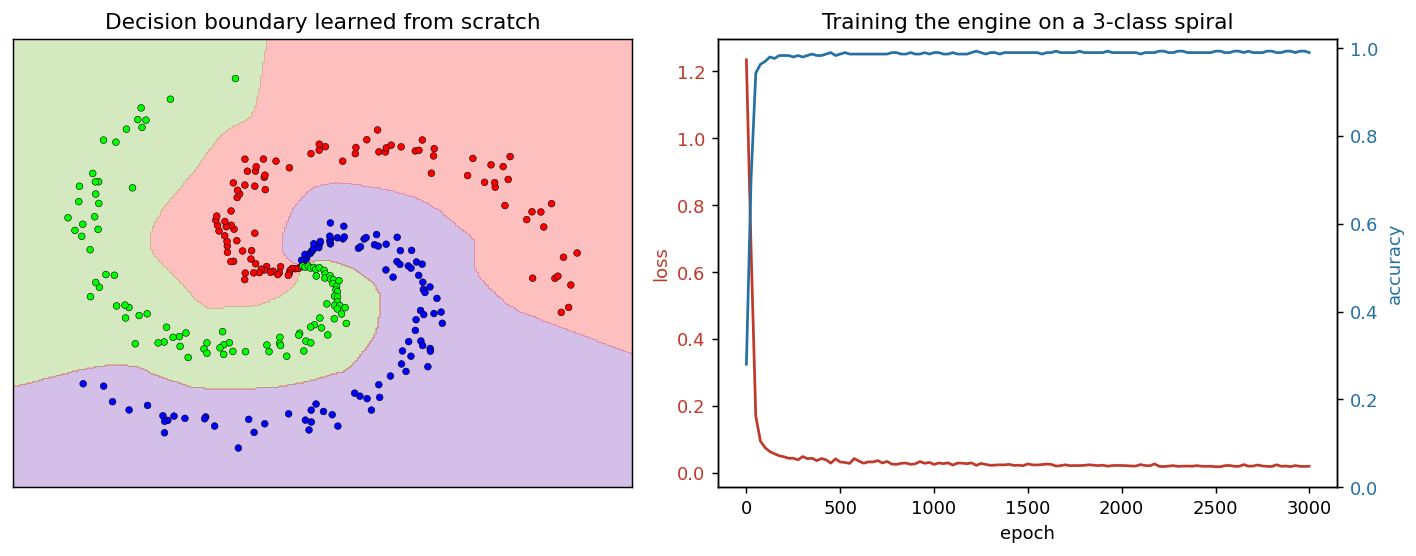
With gradients trusted, training is just three lines in a loop: forward, backward(), step. Here the engine learns a three-class spiral — a deliberately nonlinear task no linear model can separate — reaching 99.3% accuracy with a $[2,64,64,3]$ ReLU network and plain gradient descent. Every weight update in this figure was computed by the engine above, not by PyTorch.

Extensions

The engine is small on purpose — small enough to extend in an afternoon. Each of these turns it into something you'd recognize from a real framework.

1. Adam, and why it matters. Replace the plain SGD step with Adam (per-parameter adaptive moments). Plot loss-vs-epoch for both on the spiral and watch the constant-learning-rate SGD struggle where Adam glides.
2. A no_grad context. At inference you don't want the tape. Add a global flag that makes ops skip building _backward, and measure the forward-pass speedup.
3. Forward mode too. Reverse mode is cheap when outputs $\ll$ inputs (one loss, many weights). Implement forward-mode AD with dual numbers and show it wins the opposite regime — many outputs, few inputs — which is the whole reason both exist.
4. Double backprop. Make backward itself differentiable so you can take the gradient of a gradient. That single capability gives you Hessian–vector products, and with them Newton and Gauss–Newton steps.
5. A convolution op. Add conv2d with a broadcasting-correct backward, and train the same engine on a small image task. The _unbroadcast discipline is exactly what makes this tractable.
6. Visualize the tape. Walk _prev and emit Graphviz; seeing the graph of a two-layer MLP is the fastest way to understand what "the chain rule in reverse" really means.