2D Finite Difference Method

Numerical Methods

The finite difference method is a numerical technique for solving partial differential equations (PDEs) by discretizing the domain and approximating derivatives using finite differences. This page demonstrates solving the 2D Laplace equation using the Gauss-Seidel iterative method.

2D Laplace Equation

The Laplace equation in two dimensions is:

\frac{\partial ^{2} u}{\partial x ^{2}} + \frac{\partial ^{2} u}{\partial y ^{2}} = 0

This equation appears in many physical contexts, including:

Electrostatics (electric potential)
Heat conduction (steady-state temperature)
Fluid flow (stream function)
Gravitational potential

Finite Difference Discretization

Using central differences on a uniform grid with spacing $Δ x = Δ y = h$ , the second derivatives are approximated as:

\frac{\partial ^{2} u}{\partial x ^{2}} \approx \frac{u _{i + 1, j} - 2 u _{i, j} + u _{i - 1, j}}{h ^{2}}

\frac{\partial ^{2} u}{\partial y ^{2}} \approx \frac{u _{i, j + 1} - 2 u _{i, j} + u _{i, j - 1}}{h ^{2}}

Substituting into the Laplace equation and rearranging gives:

u_{i, j} = \frac{1}{4} (u_{i + 1, j} + u_{i - 1, j} + u_{i, j + 1} + u_{i, j - 1})

This is the discrete form of the Laplace equation: each interior point is the average of its four nearest neighbors.

Gauss-Seidel Iteration

The Gauss-Seidel method solves the system iteratively by updating each point using the most recent values:

u_{i, j}^{(k + 1)} = \frac{1}{4} (u_{i + 1, j}^{(k)} + u_{i - 1, j}^{(k + 1)} + u_{i, j + 1}^{(k)} + u_{i, j - 1}^{(k + 1)})

The iteration continues until convergence, typically measured by:

i, j max ∣ u_{i, j}^{(k + 1)} - u_{i, j}^{(k)} ∣ < ϵ

where $ϵ$ is a small tolerance.

Boundary Conditions

Boundary conditions must be specified. Common types include:

Dirichlet: $u = f (x, y)$ on the boundary
Neumann: $\partial u / \partial n = g (x, y)$ on the boundary
Mixed: Different conditions on different parts of the boundary

Python Implementation

The following code solves the 2D Laplace equation with various boundary conditions:

import numpy as np
import matplotlib.pyplot as plt
import matplotlib as mpl

def set_publication_style():
    """Set publication-quality matplotlib style."""
    mpl.rcParams.update({
        'font.family': 'serif',
        'font.size': 12,
        'axes.labelsize': 14,
        'axes.titlesize': 16,
        'axes.linewidth': 1.2,
        'axes.labelpad': 8,
        'axes.titlepad': 10,
        'xtick.labelsize': 12,
        'ytick.labelsize': 12,
        'xtick.direction': 'in',
        'ytick.direction': 'in',
        'xtick.top': True,
        'ytick.right': True,
        'xtick.major.size': 6,
        'ytick.major.size': 6,
        'xtick.major.width': 1.2,
        'ytick.major.width': 1.2,
        'legend.fontsize': 12,
        'legend.frameon': False,
        'lines.linewidth': 2,
        'lines.markersize': 6,
        'figure.dpi': 100,
        'savefig.dpi': 300,
        'savefig.bbox': 'tight'
    })

set_publication_style()

def solve_laplace_2d(Lx, Ly, Nx, Ny, boundary_conditions, tolerance=1e-6, max_iter=10000):
    """
    Solve the 2D Laplace equation using Gauss-Seidel iteration.
    
    Parameters:
        Lx, Ly: Domain dimensions
        Nx, Ny: Number of grid points
        boundary_conditions: Function that sets boundary values
        tolerance: Convergence tolerance
        max_iter: Maximum iterations
    
    Returns:
        u: Solution array
        iterations: Number of iterations
    """
    # Initialize solution array
    u = np.zeros((Nx, Ny))
    
    # Set boundary conditions
    boundary_conditions(u, Lx, Ly, Nx, Ny)
    
    # Gauss-Seidel iteration
    for iteration in range(max_iter):
        u_old = u.copy()
        
        # Update interior points
        for i in range(1, Nx-1):
            for j in range(1, Ny-1):
                u[i, j] = 0.25 * (u[i+1, j] + u[i-1, j] + u[i, j+1] + u[i, j-1])
        
        # Reapply boundary conditions (in case they depend on iteration)
        boundary_conditions(u, Lx, Ly, Nx, Ny)
        
        # Check convergence
        if np.max(np.abs(u - u_old)) < tolerance:
            return u, iteration + 1
    
    return u, max_iter

# Example 1: Zero boundary conditions
def zero_boundary(u, Lx, Ly, Nx, Ny):
    """All boundaries set to zero."""
    u[:, 0] = 0    # Left
    u[:, -1] = 0   # Right
    u[0, :] = 0    # Bottom
    u[-1, :] = 0   # Top

# Example 2: Mixed boundary conditions
def mixed_boundary(u, Lx, Ly, Nx, Ny):
    """Mixed boundary conditions."""
    u[:, 0] = 1.0                                    # Left: u = 1
    u[:, -1] = 0.0                                   # Right: u = 0
    u[0, :] = 0.0                                    # Bottom: u = 0
    x = np.linspace(0, Lx, Nx)
    u[-1, :] = np.sin(np.pi * x / Lx)                # Top: u = sin(πx/Lx)

# Example 3: Linear gradient
def gradient_boundary(u, Lx, Ly, Nx, Ny):
    """Linear gradient from left to right."""
    y = np.linspace(0, Ly, Ny)
    u[:, 0] = y / Ly                                 # Left: linear gradient
    u[:, -1] = y / Ly                                # Right: same gradient
    u[0, :] = 0.0                                    # Bottom: u = 0
    u[-1, :] = 1.0                                   # Top: u = 1

# Parameters
Lx, Ly = 1.0, 1.0
Nx, Ny = 50, 50

# Solve Example 1: Zero boundaries
print("Example 1: Zero boundary conditions")
u1, iter1 = solve_laplace_2d(Lx, Ly, Nx, Ny, zero_boundary)
print(f"Converged in {iter1} iterations")

# Solve Example 2: Mixed boundaries
print("\nExample 2: Mixed boundary conditions")
u2, iter2 = solve_laplace_2d(Lx, Ly, Nx, Ny, mixed_boundary)
print(f"Converged in {iter2} iterations")

# Solve Example 3: Gradient boundaries
print("\nExample 3: Gradient boundary conditions")
u3, iter3 = solve_laplace_2d(Lx, Ly, Nx, Ny, gradient_boundary)
print(f"Converged in {iter3} iterations")

# Plotting
fig, axes = plt.subplots(1, 3, figsize=(15, 5))

X, Y = np.meshgrid(np.linspace(0, Lx, Nx), np.linspace(0, Ly, Ny))

# Example 1
im1 = axes[0].contourf(X, Y, u1.T, 20, cmap='viridis')
axes[0].set_title('Zero Boundary Conditions')
axes[0].set_xlabel('x')
axes[0].set_ylabel('y')
plt.colorbar(im1, ax=axes[0], label='u(x, y)')

# Example 2
im2 = axes[1].contourf(X, Y, u2.T, 20, cmap='viridis')
axes[1].set_title('Mixed Boundary Conditions')
axes[1].set_xlabel('x')
axes[1].set_ylabel('y')
plt.colorbar(im2, ax=axes[1], label='u(x, y)')

# Example 3
im3 = axes[2].contourf(X, Y, u3.T, 20, cmap='viridis')
axes[2].set_title('Gradient Boundary Conditions')
axes[2].set_xlabel('x')
axes[2].set_ylabel('y')
plt.colorbar(im3, ax=axes[2], label='u(x, y)')

plt.tight_layout()
plt.savefig('figures/laplace_2d_solutions.png', dpi=300, bbox_inches='tight')
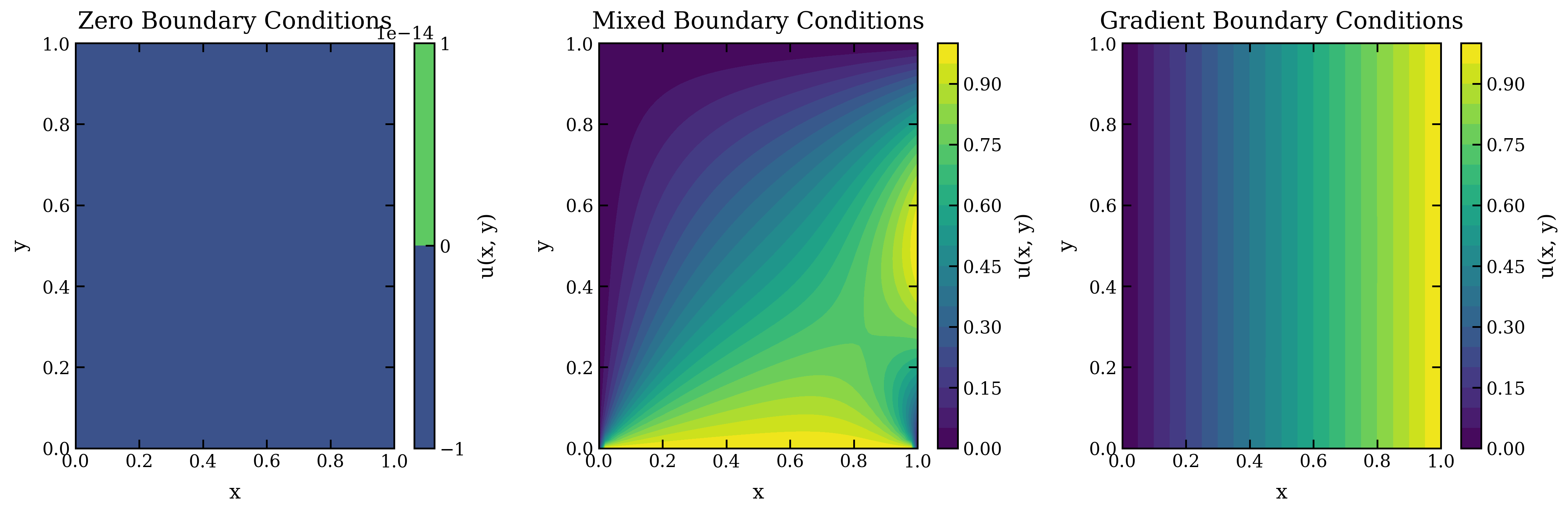
plt.show()

Visualization

The following plot shows solutions to the 2D Laplace equation with different boundary conditions:

Convergence Properties

The Gauss-Seidel method converges for the Laplace equation because:

The discrete Laplacian matrix is diagonally dominant
The spectral radius of the iteration matrix is less than 1
The method is stable for well-posed boundary value problems

The convergence rate depends on:

Grid spacing $h$ (finer grids converge slower)
Boundary conditions (smooth boundaries converge faster)
Initial guess (closer guesses require fewer iterations)

Applications

The 2D finite difference method for Laplace's equation is widely used in:

Electrostatics: Computing electric potential from charge distributions
Heat transfer: Steady-state temperature distributions
Fluid mechanics: Potential flow and stream functions
Image processing: Smoothing and denoising
Computer graphics: Surface fairing and mesh smoothing

Extensions

The method can be extended to:

Poisson equation: $\nabla^{2} u = f (x, y)$ with source term
3D problems: Using 6-point stencil instead of 4-point
Non-uniform grids: Adaptive mesh refinement
Non-linear equations: Iterative linearization