Skyrme–Hartree–Fock
Nuclear Physics
What you need to know first 8 concepts, 5 layers
The requisite-knowledge inventory for this page, bottom-up: the primitives at the base, combined upward until you reach what this page assumes. Skim the layers you already own; start wherever the ground gets unfamiliar.
- base
- Linear algebraconcept
- Quantum mechanics (states & operators)
- L1
- L2
- L3
- L4
- ↳you are here
1 of these are concepts without a dedicated page yet — the grey chips. Following the linked ones first makes the rest land.
Put protons and neutrons in a box — eight of each for oxygen-16 — and ask two questions: what arrangement do they settle into, and how much energy holds them together? This page is a from-scratch Python program that answers both, built on one approximation: each particle moves independently through the averaged push and pull of all the others. It reproduces the calculation of Vautherin & Brink (Phys. Rev. C 5, 626, 1972), the paper that launched this way of computing nuclei, and its answers are checked against measured nuclear masses and sizes from oxygen-16 up to lead-208. If you would rather build the solver than read about it, the step-by-step tutorial assembles the same program from nothing, one runnable piece at a time.
The idea, before any equations
First, names for things. Protons and neutrons are collectively nucleons. The averaged push a nucleon feels from all the others is its mean field. A single nucleon's standing-wave pattern inside that field is an orbital — the same word and the same idea as electron orbitals in an atom. And the whole scheme is called self-consistent because it closes a loop: guess how the nucleons are distributed, compute the mean field that distribution creates, find the orbitals that field allows, refill them with the nucleons, and repeat until nothing changes. Energies on this page are in MeV (mega-electron-volts — about a million times the eV scale of chemistry) and lengths in femtometers (fm, m).
The central object is the density : how many nucleons per cubic femtometer sit at each point. It is worth pinning down what kind of thing that is, because "local density" is not the opposite of "average density" in the way it may sound. An average density is one number for the whole nucleus — count the nucleons, divide by the volume, all spatial information gone (for oxygen-16, roughly ). A local density is a function: a different value at every point — at the center of oxygen-16, half that in the surface, zero outside. The solver never touches the average; everything is built from the point-by-point values.
What makes nuclei their own subject is the force. Electrons have Coulomb's law — the exact electric attraction and repulsion, known to arbitrary precision. Nucleons have no such formula; the nuclear force is short-ranged, complicated, and still an object of research. The Skyrme interaction is a deliberately simple stand-in: a short-range force chosen so that the total energy becomes a functional — a rule that takes in entire functions (here, density profiles) and returns a single number — of just three local densities. Those three are the density itself; a kinetic density that records where the orbitals wiggle the most; and a spin-orbit density that records where nucleon spins align with their orbital motion. (Each of the three gets a full section below.) An energy that depends only on densities is a density functional — this is DFT for nuclei, decades before that acronym existed.
Two more words appear constantly, so here they are up front. Isospin is bookkeeping for a near-coincidence: the proton and the neutron have almost the same mass (938.3 vs 939.6 MeV) and feel almost the same nuclear force. So treat them as two states of one particle — the nucleon — and give that two-valuedness a quantum number built exactly like spin-: the nucleon carries isospin , and its projection says proton-or-neutron. In this solver, isospin is simply the subscript threaded through everything: each species gets its own densities , its own fields, and its own copy of every equation — identical in form, differing only in the numbers (and protons add the Coulomb electric repulsion). The label starts to matter once : the force then treats neutrons and protons slightly differently — the symmetry energy — which is exactly the physics the calcium-48 rung of the validation chain below tests.
Spin-orbit is the coupling between a nucleon's spin and its orbital motion, and it is what turns "energy levels" into nuclear shell structure. A nucleon with orbital angular momentum can carry its spin aligned or anti-aligned with that motion, giving total angular momentum — and the spin-orbit term takes a different value on each (it will appear in the equations below as ):
Drag λ from 0 to 1 and watch the amber 1f₇/₂ leave its shell: at λ = 0 the 28th nucleon sits in the middle of a degenerate 1f level (no gap at all); at physical strength the aligned partner has dropped into the gap below and a shell closure at 28 exists. Read the splittings off the diagram: 1p < 1d < 1f, growing as 2ℓ+1.
So one -level splits into a pair, and the splitting grows linearly with — s-states don't split at all, and the splitting of an state is thirteen times larger than at . Two things make the nuclear version dramatic where the atomic one is a fine-structure whisper. First, the sign: in a nucleus the aligned partner is pushed down (more bound) — opposite to atoms. Second, the size: the splitting is MeV-scale, comparable to the spacing between whole shells, not a small correction to it.
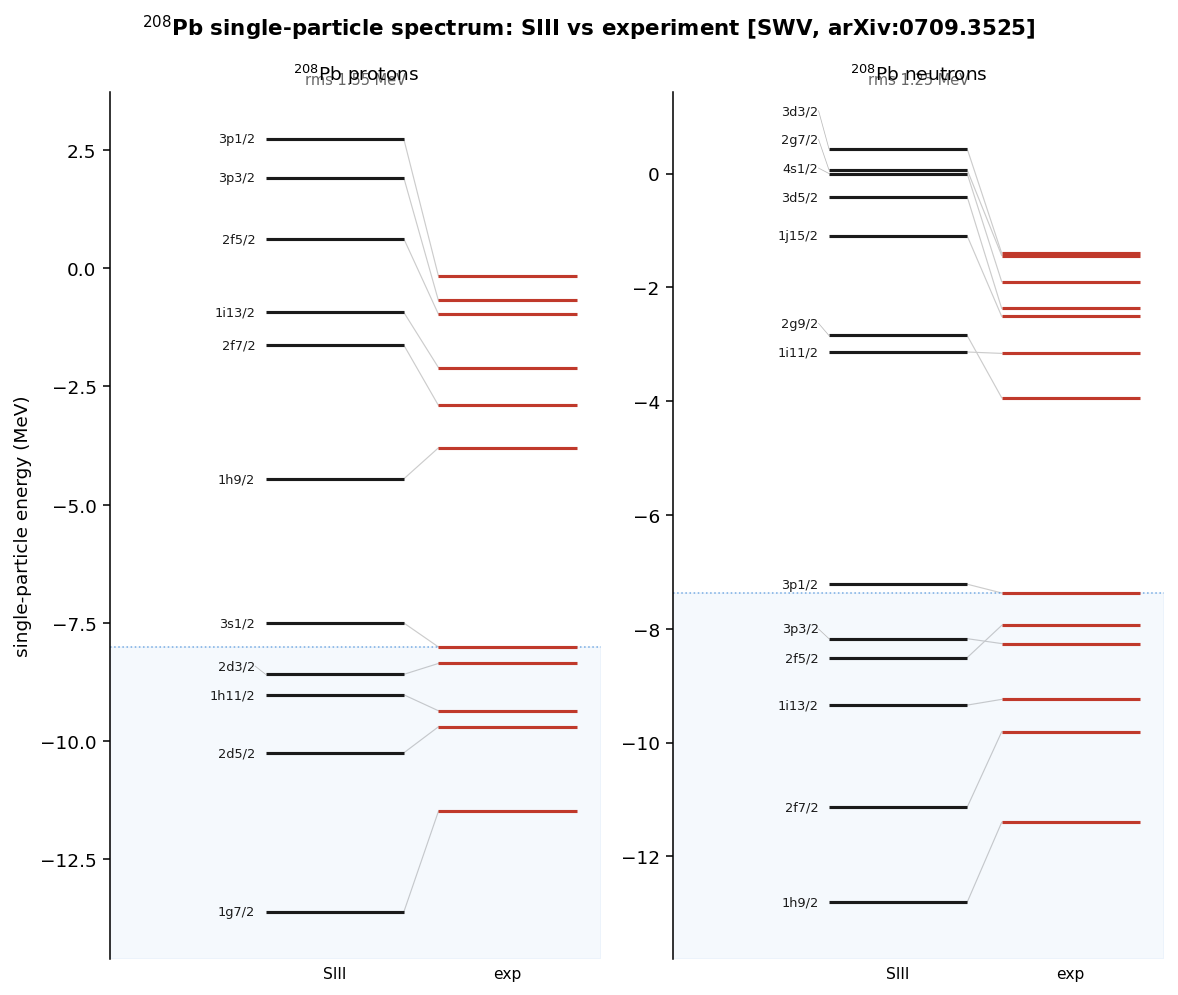
That combination rewrites the level spacings. In the spectroscopic labels used from here on, the letters s, p, d, f, g, h, i stand for and the leading number counts radial nodes. Take the highest- orbital of a shell — , , , — and the -sized kick drops its aligned member clean out of its own shell, down into the gap below: descends to create a shell closure at nucleon number 28, at 50, at 82, at 126. Without the spin-orbit term those closures would stop at 20 — and most of the nuclei this page is validated on simply wouldn't be special. That's why the lead-208 level diagram further down is a genuine test of the spin-orbit field: get it wrong and the gaps land in the wrong places.
The doubly-magic chain — why these five nuclei
Nucleons fill shells much as electrons do, and just as the noble gases sit at the closed electron shells (2, 10, 18, …), a nucleus is extra-bound when its protons or neutrons exactly fill a shell. Those counts — 2, 8, 20, 28, 50, 82, 126 — are the nuclear magic numbers (28 and above exist only because of the spin-orbit splitting described a moment ago). A nucleus is doubly-magic when both its proton number and its neutron number are magic: two shells shut at once.
That is exactly the nucleus a spherical Hartree–Fock solver can take head-on. Closed shells make the ground state spherical — so the reduction to a radial equation is exact, not an approximation — and non-degenerate, with no half-filled level to smear out. That means no pairing (the superfluid-like correlations of partly filled shells) and no deformation (non-spherical shapes) to model. They are also the best-measured nuclei on the chart. So they are where a mean-field functional has to work if it works at all: a clean pass/fail with nothing hidden in a fit parameter.
| nucleus | Z | N | shells closed | what this rung adds to the test |
|---|---|---|---|---|
| ¹⁶O | 8 | 8 | 8, 8 | Lightest doubly-magic, . The gentlest case — which is why both of the solver's bugs hid here. |
| ⁴⁰Ca | 20 | 20 | 20, 20 | Still , but 2.5× the mass — more shells filled, more of the functional exercised. |
| ⁴⁸Ca | 20 | 28 | 20, 28 | First neutron excess (). Turns on the isospin / symmetry-energy terms. The gap exists only because of spin-orbit splitting. |
| ⁹⁰Zr | 40 | 50 | 40*, 50 | Heavier, larger . is a proton sub-shell closure (semi-magic); a full magic gap. |
| ²⁰⁸Pb | 82 | 126 | 82, 126 | Heaviest known doubly-magic. Large neutron excess and large Coulomb () at once — the stringent test, and where the Coulomb bug finally showed. |
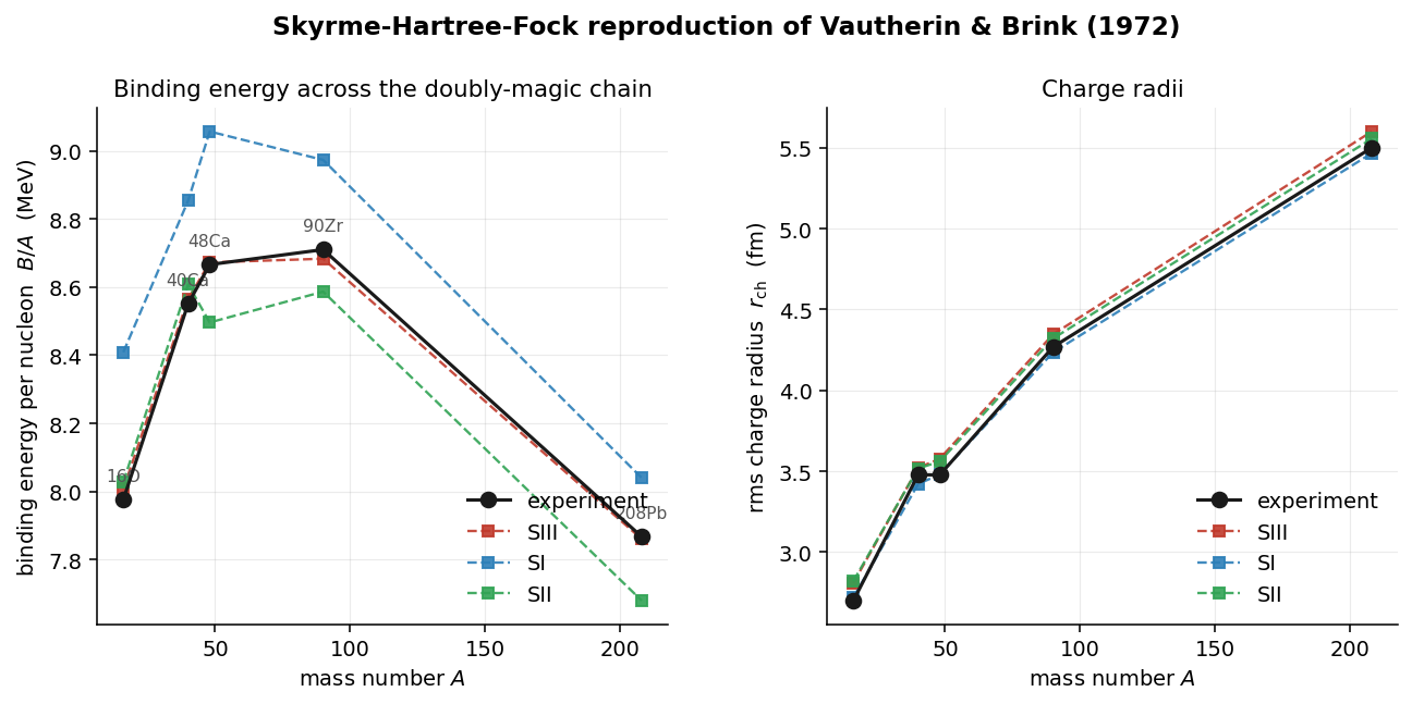
Walking the whole ladder instead of fitting one nucleus is the point: each rung turns on one new stress — more mass, then neutron excess, then heavy Coulomb. A force that reproduces all five is right for reasons that generalize, not tuned to a single point. It is also what exposes a force's character. A Skyrme force is a small set of fitted constants, and the original 1970s parameter sets are numbered SI, SII, SIII: SI over-binds the heavy end, SII under-binds it, and only SIII holds the whole chain to 0.03 MeV/A (energy per nucleon). The solver also runs two modern refits, SLy4 and SkM*, which appear in the effective-mass comparison below.
What "spherical Skyrme–Hartree–Fock" means, as equations
Let's unpack the name, one word at a time. Hartree–Fock is the many-body method: write the nucleus as a single Slater determinant — the one antisymmetric wavefunction you can build by giving every nucleon its own orbital, which is the mathematical form of "independent particles obeying the Pauli principle" — and let each nucleon move in the mean field of the others. Skyrme is the force, written not as a pair potential but as an energy that depends only on local densities. Spherical is an approximation on the field: we only allow mean fields that depend on the distance , not on direction. That is the hydrogen-atom situation — for any central potential, the angular part of every orbital is a known, pre-solved function (a spherical harmonic, the same catalog for every central problem), so the only unknown left is the radial function : a 1-D problem per . The angular momentum does not disappear — it leaves behind the centrifugal term in each radial equation, and the shell structure below is made of it. What the assumption costs is real physics: most nuclei between magic numbers are deformed (ellipsoidal), and a spherical solver cannot describe them. For our five it costs nothing, because a closed shell sums over a full multiplet to a constant — a doubly-magic density genuinely is spherical, so the assumption is self-consistent rather than imposed. Solver is the numerical engine — discretize, diagonalize, iterate. The whole program is the loop below; every box names the function in the hosted code that does it.
Hartree–Fock: minimize the energy over orbitals
The total energy is a functional of the occupied single-particle orbitals . Minimizing it, subject to the orbitals staying orthonormal, is what "self-consistent field" means:
The right-hand equation is the result that matters: varying the energy with respect to an orbital returns a Schrödinger-like eigenvalue problem for that orbital — an energy operator (a Hamiltonian) whose eigenvalue is that orbital's single-particle energy. The catch is that the operator depends on all the orbitals — so it must be solved over and over until it stops changing.
Skyrme: the energy density is a function of local densities
A real force between two nucleons has a range — it acts whenever they sit within a femtometer or two of each other. So the interaction energy is a double integral over pairs, , and the field a nucleon feels at is — a weighted sum over the density everywhere within reach. That is what nonlocal means: to get the field here you have to look at the density there, all around, and integrate. It is also expensive.
Skyrme's move is to shrink the range to zero — a contact force , dressed with a few gradient terms to fake a little width. The pair integral then collapses, , and the energy density at depends only on evaluated at that same point. No integral over neighbors: the field becomes a plain function you evaluate point by point. (This is also the second sense in which the densities are "local" — beyond being functions of position rather than one averaged number.)
Shown are the leading terms: the kinetic energy, the two-body contact term, the three-body term, and the spin-orbit term. The terms (which couple and ) and the terms are dropped here only for readability — every term is written out in total_energy(). Because is a function of the densities alone, this is a density functional — the nuclear cousin of Kohn–Sham DFT, and the same move as the LDA of electronic structure: treat each point as if it were uniform matter at that point's own density, rather than the whole system at one averaged density.
The three densities: ρ, τ, J
All three are local, per-fm³ quantities built the same way: sum over the occupied orbitals, each with its own weight. The number density weights each orbital by 1, the kinetic density by how fast it wiggles, the spin-orbit density by how much its spin aligns with its orbital motion:
The kinetic density is the local density of
kinetic energy: integrate it and you get the total,
. Why does the
force need it? Because two regions can hold the same number of nucleons
( equal) while the wavefunctions in one wiggle much more than in
the other — and a velocity-dependent interaction cares about that difference. The
gradient terms — the ones faking the force's finite width — are
exactly such couplings, and is how they enter the energy.
That coupling is also where the effective mass comes from:
picks up a -dependent piece, so
a nucleon in dense matter behaves as if it weighed less than a free one. In the
code, the spherical form is tau += w*(dR² + ℓ(ℓ+1)/r²·R²) — the
radial wiggle plus the angular wiggle that the centrifugal term encodes
(build_densities).
The spin-orbit density measures the net alignment of spin with orbital motion at each point — a spin current. Its key property is a cancellation: if both partners of a spin-orbit pair are filled, their contributions weigh in as times (the number of substates one -level holds — its degeneracy), and
so a spin-saturated system has (nearly) no at all — "nearly"
because the two partners' radial functions differ slightly once the spin-orbit
field splits them. is fed by exactly the orbitals whose
partner is empty — the high- intruders like in
— which live near the surface, so
peaks there. It then feeds back into the spin-orbit field
(): spin-aligned motion at the surface deepens the
potential that favors spin-aligned motion. In the code the spherical reduction is
one line: J += w·⟨σ·l⟩/r·R².
From energy density to mean fields
Where do the fields actually come from? They are the energy density, differentiated. The single-particle equation is ; since and every density is built from the orbitals (, , and from ), the chain rule turns each derivative-of-a-density into a mean field:
The -derivative multiplies and becomes the central potential . The -derivative sits between the two gradients of the kinetic term and becomes the effective-mass operator — so is literally . The -derivative becomes the spin-orbit field . And because is an ordinary function of the densities — not an integral over them — each derivative is again an ordinary function, evaluated point by point. That is the local field, made concrete.
Take the simplest term to watch it work. Differentiate the contact energy with respect to , remembering that so :
— which is exactly the first line of U_central in the code. Every other term is the same operation, just messier. The pieces differentiated with respect to give the density-dependent effective mass — and the minus sign on the part of , the one the sign bug got wrong, is nothing but the that falls straight out of this derivative.
The single-particle equation, reduced to a radius
Drop those fields into the single-particle equation. For a spherical nucleus every one of them depends only on , so the orbital separates into a known angular factor times an unknown radial one, — where is the standard angular function of any central-potential problem (hydrogen included) and the spin part — and the 3-D equation collapses to a single radial ODE for :
Every bracket here is a line of code. Put on a mesh and this
becomes a symmetric tridiagonal matrix — nonzero only on the
main diagonal and the two beside it, because a second derivative on a mesh
couples each point only to its immediate neighbors
(step 2 of the tutorial
builds this matrix from nothing and solves it). The centrifugal
, the potentials , and the
spin-orbit
sit on the diagonal, the effective-mass term
supplies the off-diagonals — assembled in
solve_block (the diag
and off arrays) and handed to numpy.linalg.eigh. The
spin-orbit strength is the
from the opening section.
Self-consistency closes the loop
The fields need the densities; the densities are built from the very orbitals the fields produce:
So the whole calculation is a fixed-point iteration — the loop from the top of the page, now with every step named: guess densities → build the fields → diagonalize for orbitals → rebuild the densities → mix and repeat until the energy stops moving ( and follow the same pattern with derivative and weights). That loop is the entire method; everything below is how to make each step fast and stable.
Method
The original 1972 paper expanded the orbitals in a harmonic-oscillator
basis — writing each unknown orbital as a sum over a fixed family of analytic
oscillator functions. This solver instead works directly on a radial mesh
( fm, fm, energies
grid-converged to under 0.1 MeV) and diagonalizes. Each
channel decouples into its own
symmetric tridiagonal Hamiltonian, solved with numpy.linalg.eigh;
self-consistency is reached by linear mixing of the densities between
iterations.
Why a mesh instead of an oscillator basis?
The 1972 choice was a hardware compromise. Harmonic-oscillator orbitals have closed-form matrix elements, so you can assemble the Hamiltonian without ever diagonalizing a large matrix — decisive when a large matrix was expensive. That advantage has evaporated, and for this problem the mesh wins on three counts.
The equation you actually solve is one-dimensional. As the
radial reduction above showed, a spherical nucleus leaves one 1-D equation per
channel. On a grid of a few hundred
points each of those is a small tridiagonal matrix, and a single
numpy.linalg.eigh returns every orbital in that channel at once —
energies and radial shapes together. No 3-D grid to fill, no basis set to
expand: the only thing left to converge is the grid spacing.
Skyrme is a local functional. Its entire reason for existing is that the energy depends only on local densities , so the mean field collapses to a handful of local potentials . Real space is its native habitat: you read the potentials straight off the densities, with no two-body matrix elements or Moshinsky brackets (the angular-momentum recoupling coefficients that finite-range matrix elements require) to evaluate. A finite-range force like Gogny, whose field is genuinely nonlocal, is where an oscillator basis is the right tool.
The tail comes out right for free. An oscillator orbital decays as a Gaussian, ; a real bound nucleon decays exponentially, . The oscillator basis therefore mis-describes the surface and tail until you pile on many shells — and it is exactly the surface that sets the density falloff and the charge radius (the measured size of the proton distribution). On a box the wavefunction simply decays however the potential dictates, so the exponential tail is exact. Convergence is then one monotone knob (grid spacing and box size, here to under 0.1 MeV) instead of the oscillator's two-parameter optimize-and-extrapolate.
The one subtlety is the effective mass. Skyrme forces make a nucleon's inertia position-dependent — the kinetic term becomes with set by the local density. Discretized naively it is not symmetric, and a non-Hermitian Hamiltonian gives complex energies. Keeping it in divergence form and averaging to the half-points restores exact symmetry on the uniform mesh:
def solve_block(grid, l, sig_dot_l, B, U, W, Vcoul_or_zero, nstates):
    """Diagonalize the radial HF Hamiltonian; return (eps, R)."""
    r = grid.r; h = grid.h; Nn = grid.N
    # half-point effective mass (self-adjoint divergence form, Hermitized)
    Bpad = np.empty(Nn+2)
    Bpad[1:-1] = B; Bpad[0] = B[0]; Bpad[-1] = HBAR2_2M
    Bhalf = 0.5*(Bpad[:-1] + Bpad[1:])      # B_{i-1/2}, B_{i+1/2}
    Bm = Bhalf[:-1]; Bp = Bhalf[1:]

    diag = (Bm + Bp)/h**2 \
        + B*l*(l+1)/r**2 \
        + U + Vcoul_or_zero \
        + sig_dot_l * W / r
    off = -Bp[:-1]/h**2                     # symmetric coupling i, i+1

    H = np.diag(diag) + np.diag(off, 1) + np.diag(off, -1)
    eps, vec = np.linalg.eigh(H)            # each (l,j,isospin) block: tridiagonal
    u = vec / np.sqrt(h)
    return eps[:nstates], (u / r[:, None])[:, :nstates]
Densities and single-particle spectra
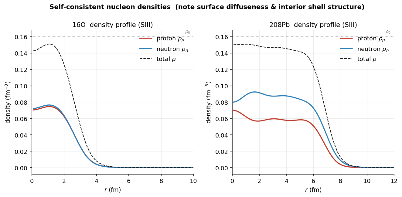
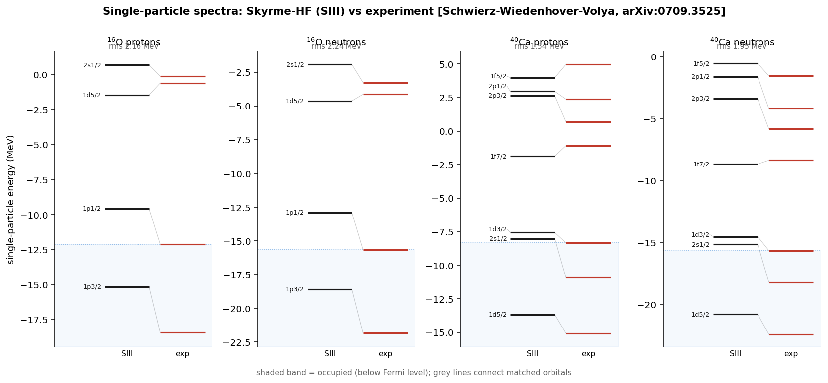
Diagonalizing the converged mean field also hands over the single-particle levels — the shell structure. Against the Schwierz–Wiedenhöver–Volya compilation of experimental single-particle energies, the root-mean-square deviation is ~1–2 MeV, with the level ordering, shell gaps, and spin-orbit splittings all in the right place.
The effective mass controls the level spacing
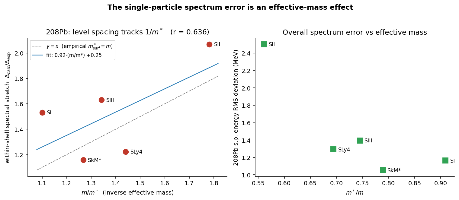
The residual ~1–2 MeV spread in the single-particle spectra is not random — it tracks the effective mass introduced above, the parameter that sets how tightly the levels bunch. The solver reproduces the published effective masses of nuclear matter (the idealized infinite medium of nucleons at uniform density that serves as every force's calibration point) across all five forces:
| force | (this solver) | literature |
|---|---|---|
| SII | 0.561 | 0.58 |
| SLy4 | 0.694 | 0.69 |
| SIII | 0.745 | 0.76 |
| SkM* | 0.789 | 0.79 |
| SI | 0.909 | ~0.91 |
Comparing five different forces at once is noisy — each one changes the whole mean field, not just the mass, so the trend is real but scattered:
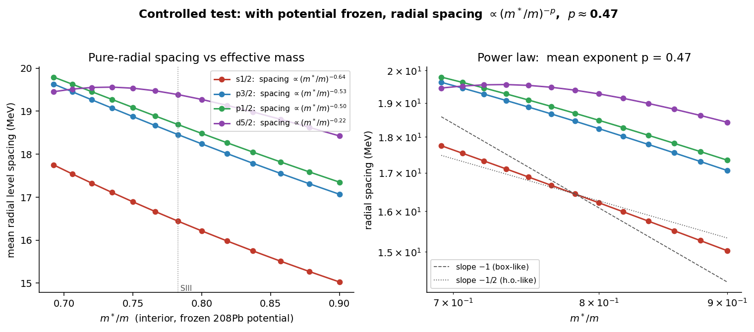
The clean test freezes the potential and scales only the effective-mass term. Then the pure-radial level spacing obeys
exactly the harmonic-oscillator scaling . A lighter effective mass spreads the shells apart; a heavier one packs them together. That pins the residual spectral discrepancy on the effective mass quantitatively, rather than leaving it as unexplained scatter.
Two bugs, both invisible on oxygen
A reproduction is only as trustworthy as the mistakes it survives. Two sign- and-scale errors passed every check and only surfaced further up the chain — a useful reminder that the light doubly-magic nucleus is a weak test.
The sign in the effective mass. The like-particle term had a where the functional derivative of the energy density gives ; the coefficient is , not . SI has a small , so oxygen looked fine — but the error wrecked SII, which has a large one. It was caught by cross-checking the nuclear-matter against the published 0.58.
Direct Coulomb. A stray cumulative-sum subtraction pushed the direct Coulomb potential negative in the surface region, making the Coulomb energy come out roughly 4× too small. The error scales as , so was untouched while over-bound by +2.2 MeV/A and its protons sat ~14 MeV too deep relative to neutrons — the tell that fingered it. Rewritten as a clean inner/outer partition and checked against the analytic uniform-sphere result (976 vs 968 MeV).
Residuals not swept aside
- Charge radii run ~0.1 fm large everywhere (worst at ) — a proton form-factor folding convention (smearing the point-proton density by the proton's own finite size) plus the missing center-of-mass correction to the radius. Not chased down.
- Some spin-orbit splittings are over-predicted — known SIII behavior.
- Validated against experiment, not Vautherin & Brink's original Table I (paywalled).
Code & references
The full solver — forces, densities, mean fields, the self-consistent-field
loop, energy and radii — is
scripts/projects/skyrme-hf-vb/skyrme_hf.py in this
repository, with driver scripts that regenerate every figure above
(test_chain.py, make_plots.py,
make_levels.py, mstar_controlled.py). Requires only
numpy and matplotlib. To build the whole thing yourself, one working step at a
time, use the
Build Your Own Nuclear DFT
tutorial — its final step is this solver.
- D. Vautherin, D. M. Brink, Phys. Rev. C 5, 626 (1972).
- Xayavong, Smirnova, arXiv:2111.13531 — derivation of the VB equations.
- Schwierz, Wiedenhöver, Volya, arXiv:0709.3525 — experimental s.p. energies.
- Chabanat et al., Nucl. Phys. A 635, 231 (1998) — SLy4.
- Bartel et al., Nucl. Phys. A 386, 79 (1982) — SkM*.