Numerov's Method

Differential Equations

Background

The Numerov method can be used for functions of the form

\frac{d ^{2} y}{d x ^{2}} = g (x) y (x) + s (x)

Steps

Taylor expand the general differential equation
Apply to discrete space
Use forward and backward step to cancel odd terms
Do some mathematical magic to get it in "nice" terms

y^{''} = g (x) y (x) + s (x)

Begin by using the formula for a Taylor expansion.

y (x) = y (x_{0}) + (x - x_{0}) y^{'} (x_{0}) + \frac{( x - x _{0} ) ^{2}}{2 !} y^{''} (x_{0}) + \frac{( x - x _{0} ) ^{3}}{3 !} y^{'''} (x_{0}) + \frac{( x - x _{0} ) ^{4}}{4 !} y^{''''} (x_{0}) + \frac{( x - x _{0} ) ^{5}}{5 !} y^{'''''} (x_{0}) + O (h^{6})

Set $x = x_{0} + h$ and $h = x - x_{0}$ leaving us with:

y (x_{0} + h) = y (x_{0}) + h y^{'} (x_{0}) + \frac{h ^{2}}{2 !} y^{''} (x_{0}) + \frac{h ^{3}}{3 !} y^{'''} (x_{0}) + \frac{h ^{4}}{4 !} y^{''''} (x_{0}) + \frac{h ^{5}}{5 !} y^{'''''} (x_{0}) + O (h^{6})

We now discretize the space using the following rule $h = x_{n + 1} - x_{n}$ . If we plug in $n = 0$ we get $h = x_{1} - x_{0}$ and consequently $x_{1} = x_{0} + h$ . This means we can rewrite $y (x_{0} + h)$ as $y (x_{1})$ :

y (x_{1}) = y (x_{0}) + h y^{'} (x_{0}) + \frac{h ^{2}}{2 !} y^{''} (x_{0}) + \frac{h ^{3}}{3 !} y^{'''} (x_{0}) + \frac{h ^{4}}{4 !} y^{''''} (x_{0}) + \frac{h ^{5}}{5 !} y^{'''''} (x_{0}) + O (h^{6})

Where we adopt the shorthand that $y (x_{n}) = y_{n}$ , giving us:

y_{1} = y_{0} + h y^{'} (x_{0}) + \frac{h ^{2}}{2 !} y^{''} (x_{0}) + \frac{h ^{3}}{3 !} y^{'''} (x_{0}) + \frac{h ^{4}}{4 !} y^{''''} (x_{0}) + \frac{h ^{5}}{5 !} y^{'''''} (x_{0}) + O (h^{6})

From this we make the observation that:

y_{n + 1} = y_{n} + h y^{'} (x_{n}) + \frac{h ^{2}}{2 !} y^{''} (x_{n}) + \frac{h ^{3}}{3 !} y^{'''} (x_{n}) + \frac{h ^{4}}{4 !} y^{''''} (x_{n}) + \frac{h ^{5}}{5 !} y^{'''''} (x_{n}) + O (h^{6})

Similarly, if we want to take a step backwards we can replace every $h$ with $- h$ :

y_{n - 1} = y_{n} - h y^{'} (x_{n}) + \frac{h ^{2}}{2 !} y^{''} (x_{n}) - \frac{h ^{3}}{3 !} y^{'''} (x_{n}) + \frac{h ^{4}}{4 !} y^{''''} (x_{n}) - \frac{h ^{5}}{5 !} y^{'''''} (x_{n}) + O (h^{6})

The odd terms are the only ones that change sign. Next, we can add the two expressions together and rearranging:

y_{n + 1} - 2 y_{n} + y_{n - 1} = + h^{2} y_{n}^{''} + \frac{h ^{4}}{12} y_{n}^{''''} + O (h^{6})

From the statement of the problem $y^{''} (x) = - g (x) y (x) + s (x)$ , we have $y_{n}^{''} = - g_{n} y_{n} + s_{n}$ . So in continuous variables we have:

y^{''''} (x) = \frac{d ^{2}}{d x ^{2}} (- g (x) y (x) + s (x))

and in discrete variables we have:

y_{n}^{''''} = \frac{d ^{2}}{d x ^{2}} (g_{n} y_{n} + s_{n})

Remember that the second derivative can be approximated as a finite difference scheme:

f^{''} (x) \approx \frac{\frac{f ( x + h ) - f ( x )}{h} - \frac{f ( x ) - f ( x - h )}{h}}{h} = \frac{f ( x + h ) - 2 f ( x ) + f ( x - h )}{h ^{2}} .

Let $f (x + h) = g (x + h) y (x + h) + s (x + h)$ , $f (x) = g (x) y (x) + s (x)$ , and $f (x - h) = g (x - h) y (x - h) + s (x - h)$ . Now plug these terms into the finite difference scheme:

y^{''''} (x) = f^{''} (x) = \frac{g ( x + h ) y ( x + h ) + s ( x + h ) + 2 g ( x ) y ( x ) - 2 s ( x ) + g ( x - h ) y ( x - h ) + s ( x - h )}{h ^{2}}

Converting to discrete space:

y_{n}^{''''} = \frac{g _{n + 1} y _{n + 1} + s _{n + 1} + 2 g _{n} y _{n} - 2 s _{n} + g _{n - 1} y _{n - 1} + s _{n - 1}}{h ^{2}}

Now that we have an expression for $y_{n}^{''''}$ we can substitute this back into:

y_{n + 1} - 2 y_{n} + y_{n - 1} = h^{2} y_{n}^{''} + \frac{h ^{4}}{12} y_{n}^{''''} + O (h^{6})

leaving the following equation:

y_{n + 1} - 2 y_{n} + y_{n - 1} = h^{2} y_{n}^{''} + \frac{h ^{4}}{12} (\frac{- g _{n + 1} y _{n + 1} + s _{n + 1} + 2 g _{n} y _{n} - 2 s _{n} + g _{n - 1} y _{n - 1} + s _{n - 1}}{h ^{2}}) + O (h^{6})

Cancelling $h^{2}$ :

y_{n + 1} - 2 y_{n} + y_{n - 1} = h^{2} y_{n}^{''} + \frac{h ^{2}}{12} (g_{n + 1} y_{n + 1} + s_{n + 1} + 2 g_{n} y_{n} - 2 s_{n} + g_{n - 1} y_{n - 1} + s_{n - 1}) + O (h^{6})

This is a very unwieldy expression so let's try to see if we can pull together some common terms with subscript $n + 1$ , $n$ and $n - 1$ . The right side has the same form as the finite difference formula, we can probably match these terms up with the $y_{n + 1} - 2 y_{n} + y_{n - 1}$ :

y_{n + 1} - 2 y_{n} + y_{n - 1} = h^{2} y_{n}^{''} + \frac{h ^{2}}{12} (g_{n + 1} y_{n + 1} + s_{n + 1} - 2 g_{n} y_{n} - 2 s_{n} + g_{n - 1} y_{n - 1} + s_{n - 1}) + O (h^{6})

[y_{n + 1} - \frac{h ^{2}}{12} (g_{n + 1} y_{n + 1}) - \frac{h ^{2}}{12} (s_{n + 1})] + 2 [- y_{n} + \frac{h ^{2}}{12} (g_{n} y_{n}) + \frac{h ^{2}}{12} (s_{n})] + [y_{n - 1} - \frac{h ^{2}}{12} (g_{n - 1} y_{n - 1}) - \frac{h ^{2}}{12} (s_{n - 1})] = h^{2} y_{n}^{''} + O (h^{6})

The first bracketed term

[y_{n + 1} - \frac{h ^{2}}{12} g_{n + 1} y_{n + 1} - \frac{h ^{2}}{12} s_{n + 1}]

becomes

[y_{n + 1} (1 - \frac{h ^{2}}{12} g_{n + 1}) - \frac{h ^{2}}{12} s_{n + 1}]

The second bracketed term

2 [- y_{n} + \frac{h ^{2}}{12} g_{n} y_{n} + \frac{h ^{2}}{12} s_{n}]

becomes

- 2 [y_{n} (1 - \frac{h ^{2}}{12} g_{n}) - \frac{h ^{2}}{12} s_{n}]

and finally

[y_{n - 1} - \frac{h ^{2}}{12} (g_{n - 1} y_{n - 1}) - \frac{h ^{2}}{12} (s_{n - 1})]

becomes

[y_{n - 1} (1 - \frac{h ^{2}}{12} g_{n - 1}) - \frac{h ^{2}}{12} s_{n - 1}]

Each of these similar terms can be absorbed into a new variable $w_{n}$ :

w_{n} = y_{n} (1 - \frac{h ^{2}}{12} g_{n}) - \frac{h ^{2}}{12} s_{n}

simplifying our unwieldy expression to:

w_{n + 1} - 2 w_{n} + w_{n - 1} = h^{2} y_{n}^{''} + O (h^{6})

Substituting $y_{n}^{''} = g_{n} y_{n} + s_{n}$ , we arrive at our final answer:

w_{n + 1} - 2 w_{n} + w_{n - 1} = h^{2} (g_{n} y_{n} + s_{n}) + O (h^{6})

We need to remember that:

y_{n} = \frac{w _{n} + \frac{h ^{2}}{12} s _{n}}{1 - \frac{h ^{2}}{12} g _{n}}

Practical Considerations

To implement the method there are a few practical considerations, for example:

How do we start the calculation method without knowing the value of the first step?

We take two small values and set them equal to $y_{0}$ and $y_{1}$ , let $y_{0} = 0$ and $y_{1} = 0.001$ . Then:

w_{0} = y_{0} (1 - \frac{h ^{2}}{12} g_{0}) - \frac{h ^{2}}{12} s_{0}

w_{1} = y_{1} (1 - \frac{h ^{2}}{12} g_{1}) - \frac{h ^{2}}{12} s_{1}

So now we have taken the first two steps and can use this formula:

w_{n + 1} = 2 w_{n} - w_{n - 1} + h^{2} (g_{n} y_{n} + s_{n})

for the case $w_{2} = 2 w_{1} - w_{0} + h^{2} (g_{1} y_{1} + s_{1})$ .

In short, you need to give the Numerov method the first and second step, the first step can be zero and the second step should be a small positive number.

Simplified Numerov

Numerov's Method can be simplified for differential equations where $s (x) = 0$ , giving:

y^{''} = g (x) y (x)

The $w$ term simply loses the $s$ terms.

Generalized Numerov

Note: these routines were taken directly from Kristjan Haule's LAPW code

Numerov's method presumes that the differential equation is of the form:

\frac{d ^{2} y}{d x ^{2}} = g (x) y (x)

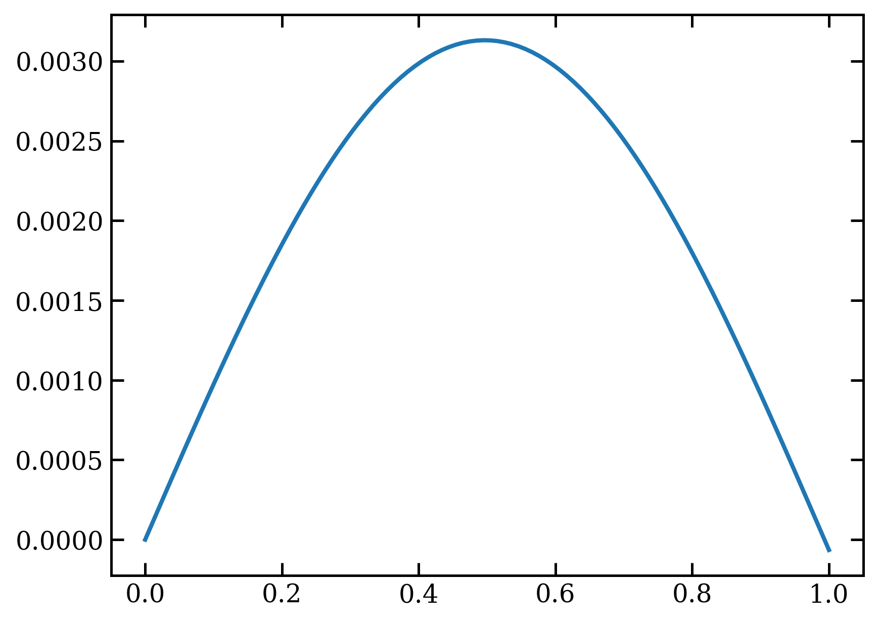
Which is not too far off from the infinite square well hamiltonian, with the function $g (x)$ actually being a constant $- \frac{2 m E}{h ^{2}}$ :

\frac{d ^{2}}{d x ^{2}} ψ (x) = - \frac{2 m E}{h ^{2}} ψ (x)

Feel free to mess with the "constant" to change the result. Note that this is not a valid wavefunction because it is not normalized.

import numpy as np
import matplotlib.pyplot as plt
import matplotlib as mpl

def set_publication_style():
    """Set publication-quality matplotlib style."""
    mpl.rcParams.update({
        'font.family': 'serif',
        'font.size': 12,
        'axes.labelsize': 14,
        'axes.titlesize': 16,
        'axes.linewidth': 1.2,
        'axes.labelpad': 8,
        'axes.titlepad': 10,
        'xtick.labelsize': 12,
        'ytick.labelsize': 12,
        'xtick.direction': 'in',
        'ytick.direction': 'in',
        'xtick.top': True,
        'ytick.right': True,
        'xtick.major.size': 6,
        'ytick.major.size': 6,
        'xtick.major.width': 1.2,
        'ytick.major.width': 1.2,
        'legend.fontsize': 12,
        'legend.frameon': False,
        'lines.linewidth': 2,
        'lines.markersize': 6,
        'figure.dpi': 100,
        'savefig.dpi': 300,
        'savefig.bbox': 'tight'
    })

set_publication_style()

# Simplified Numerov (for s(x) = 0)
def Numerov(F, dx, f0=0.0, f1=1e-3):
    Nmax = len(F)
    dx = float(dx)
    Solution = np.zeros(Nmax, dtype=float)
    Solution[0] = f0
    Solution[1] = f1
    h2 = dx*dx;
    h12 = h2/12;
      
    w0 = (1-h12*F[0])*Solution[0];
    Fx = F[1];
    w1 = (1-h12*Fx)*Solution[1];
    Phi = Solution[1];
      
    w2 = 0.0
    for i in range(2, Nmax):
        w2 = 2*w1 - w0 + h2*Phi*Fx;
        w0 = w1;
        w1 = w2;
        Fx = F[i];
        Phi = w2/(1-h12*Fx);
        Solution[i] = Phi;
    return Solution

# Generalized Numerov (for s(x) != 0)
def NumerovGen(F, U, dx, f0=0.0, f1=1e-3):
    Nmax = len(F)
    dx = float(dx)
    Solution = np.zeros(Nmax, dtype=float)
    Solution[0] = f0
    Solution[1] = f1

    h2 = dx * dx
    h12 = h2 / 12

    w0 = Solution[0] * (1 - h12 * F[0]) - h12 * U[0]
    w1 = Solution[1] * (1 - h12 * F[1]) - h12 * U[1]
    Phi = Solution[1]

    for i in range(2, Nmax):
        Fx = F[i]
        Ux = U[i]
        w2 = 2 * w1 - w0 + h2 * (Phi * Fx + Ux)
        w0 = w1
        w1 = w2
        Phi = (w2 + h12 * Ux) / (1 - h12 * Fx)
        Solution[i] = Phi

    return Solution

# Example usage: Infinite square well
constant = -10.0
x = np.linspace(0,1,100)
isw_rhs = constant*np.ones(len(x))

sol = Numerov(isw_rhs, x[1]-x[0], 0.00, 0.0001)

plt.plot(x, sol)
plt.savefig('figures/numerov_solution.png', dpi=300, bbox_inches='tight')
plt.show()

Visualization

The following plot shows the solution obtained using Numerov's method:

C++ Implementation

The following C++ code implements both standard and generalized Numerov methods:

#include <vector>
#include <cmath>
#include <iostream>

// Helper function: linspace
std::vector<double> linspace(double start, double end, size_t num) {
    std::vector<double> result(num);
    double dx = (end - start) / (num - 1);
    for (size_t i = 0; i < num; ++i) {
        result[i] = start + i * dx;
    }
    return result;
}

// Coulomb potential
double coulombPotential(double r, double Z) {
    if (r < 1e-10) return 0.0;  // Avoid singularity
    return -Z / r;
}

/* =======================
   Standard Numerov
   ======================= */
std::vector<double>
Numerov(const std::vector<double>& F,
        double dx,
        double f0,
        double f1)
{
    const std::size_t Nmax = F.size();

    std::vector<double> Solution(Nmax, 0.0);
    Solution[0] = f0;
    Solution[1] = f1;

    const double h2  = dx * dx;
    const double h12 = h2 / 12.0;

    double w0 = (1.0 - h12 * F[0]) * Solution[0];
    double Fx = F[1];
    double w1 = (1.0 - h12 * Fx) * Solution[1];
    double Phi = Solution[1];

    for (std::size_t i = 2; i < Nmax; ++i)
    {
        double w2 = 2.0 * w1 - w0 + h2 * Phi * Fx;

        w0 = w1;
        w1 = w2;

        Fx = F[i];
        Phi = w2 / (1.0 - h12 * Fx);
        Solution[i] = Phi;
    }

    return Solution;
}

/* =======================
   Generalized Numerov
   ======================= */
std::vector<double>
NumerovGen(const std::vector<double>& F,
           const std::vector<double>& U,
           double dx,
           double f0,
           double f1)
{
    const std::size_t Nmax = F.size();

    std::vector<double> Solution(Nmax, 0.0);
    Solution[0] = f0;
    Solution[1] = f1;

    const double h2  = dx * dx;
    const double h12 = h2 / 12.0;

    double w0 = Solution[0] * (1.0 - h12 * F[0]) - h12 * U[0];
    double w1 = Solution[1] * (1.0 - h12 * F[1]) - h12 * U[1];
    double Phi = Solution[1];

    for (std::size_t i = 2; i < Nmax; ++i)
    {
        const double Fx = F[i];
        const double Ux = U[i];

        double w2 = 2.0 * w1 - w0 + h2 * (Phi * Fx + Ux);

        w0 = w1;
        w1 = w2;

        Phi = (w2 + h12 * Ux) / (1.0 - h12 * Fx);
        Solution[i] = Phi;
    }

    return Solution;
}

// Radial Schrödinger equation RHS
std::vector<double> radialRHS(
    double E,
    double l,
    const std::vector<double>& R,
    const std::vector<double>& Veff
) {
    const std::size_t N = R.size();
    std::vector<double> RHS(N, 0.0);

    for (std::size_t i = 0; i < N; ++i) {
        double r = R[i];
        if (r < 1e-10) r = 1e-10;  // Avoid division by zero
        RHS[i] = 2.0 * (-E + 0.5 * l * (l + 1.0) / (r * r) + Veff[i]);
    }

    return RHS;
}

// Example usage for radial Schrödinger equation
int main() {
    std::vector<double> r = linspace(0.01, 20.0, 10000);  // Start slightly away from origin
    std::vector<double> Veff(r.size());

    // Set up potential (e.g., Coulomb potential for hydrogen)
    for (size_t i = 0; i < Veff.size(); i++) {
        Veff[i] = coulombPotential(r[i], 1.0);  // Z = 1
    }

    // Compute RHS for given energy E and angular momentum l
    double E = -0.5;  // Energy in atomic units
    double l = 0.0;   // Angular momentum quantum number
    std::vector<double> rhs = radialRHS(E, l, r, Veff);

    // Solve using Numerov
    double dx = r[1] - r[0];
    std::vector<double> solution = Numerov(rhs, dx, 0.0, 1e-3);

    // Print some results
    std::cout << "Solution at r=0.01: " << solution[0] << std::endl;
    std::cout << "Solution at r=1.0: " << solution[100] << std::endl;
    std::cout << "Solution at r=10.0: " << solution[5000] << std::endl;

    return 0;
}