Adomian Decomposition

Differential Equations

The Adomian Decomposition is a systematic method for solving differential equations.

The Adomian Decomposition is related to a variety of different concepts. Concepts which, in my estimation, are necessary to understand the method as a whole.

Picard Iteration
Operator Form of Differential Equations
Generating Functions
Taylor Series
Power Series
Absolute Convergence
Radius of Convergence
Faà di Bruno
Adomian Polynomials

Understanding any one of these concepts on its own is an endeavor, but applying them all at once in the Adomian Decomposition can make it difficult to understand. It is my hope that by separating the components in the Adomian Decomposition the method becomes clear and you are able to apply the method to your own problems.

An Introduction to the Adomian Decomposition Method

We can write differential equations in operator form. The particular form which we will use is

L [u] + R [u] + N [u] = f (x)

We will take the differential equation

\frac{d u}{d x} + sin (x) u + e^{u} = x^{2}

and associate each term of the equation with the operator form above.

L [u] = \frac{d}{d x} [u], R [u] = sin (x) u, N [u] = e^{u}, f (x) = x^{2}

L stands for Linear invertible, R stands for remainder, and N stands for nonlinear. $f (x)$ is the inhomogeneous term. If we do some re-arranging:

L [u] = - R [u] - N [u] + f (x)

We can apply the L inverse operator and simplify to:

u = L^{- 1} [- R [u] - N [u] + f (x)]

Well, this is all good and all, but what exactly is the L inverse operator? To explore this idea, let's side-step to a simpler problem.

A simpler problem

This is the level 0 of differential equations, which is an appropriate place to start.

\frac{d u}{d x} = u u (0) = 1

Rewriting the equation:

\frac{d}{d x} [u] = u u (0) = 1

We now have to choose again how we would like to represent the expression. To avoid confusion with our first example I have added subscripts.

L_{1} [u] = \frac{d}{d x} [u], R_{1} [u] = - I u, N_{1} [u] = 0, f_{1} (x) = 0

I is defined as the identity matrix. This is strictly not necessary, but it is here to show that there is an operator acting on u. It also shows the non-invertible portion of the operator: the inverse of the identity is the identity, so it doesn't get us very far if we wanted to solve using R inverse. Since we can invert the differentiation, we will go with that.

u = L_{1}^{- 1} R_{1} [u]

Which can be written as:

\int_{x_{0}}^{x} \frac{d}{d x} [u] d x = \int_{x_{0}}^{x} u d x

Which turns into:

u (x) - u (x_{0}) = \int_{x_{0}}^{x} u d x

This can be interpreted as an iterative scheme:

u_{n + 1} = u_{0} + \int_{0}^{x} u_{n} d x

which is known as the "Picard Iteration", "method of successive approximations", or a "fixed-point iteration". Why so many names? The Picard iteration is the most specific to differential equations, and the other two are more general terms.

These iterations are known to be robust, but not very fast. In the context of integration specifically it is commonly known as a Picard iteration. Picard iterations can be used to prove the existence of a solution to a differential equation. Back to the problem: we have converted a differential equation into an integral equation, now let's start iterating.

u_{0} = 1

u_{1} = 1 + \int_{0}^{x} d x = 1 + x

u_{2} = 1 + \int_{0}^{x} (1 + x) d x = 1 + x + \frac{x ^{2}}{2}

u_{3} = 1 + \int_{0}^{x} (1 + x + \frac{x ^{2}}{2}) d x = 1 + x + \frac{x ^{2}}{2} + \frac{x ^{3}}{3 !}

A pattern is starting to emerge.

u_{n} = k = 0 \sum n \frac{x ^{k}}{k !}

The Adomian Version

The previous solution has an interesting character to it: the nth iteration is the nth estimate. What if we re-wrote the series in a way where the sum of n terms becomes the nth estimate? Rewriting the problem like this is not too difficult.

u_{0} = u_{0}

u_{n + 1} = \int_{0}^{x} u_{n} d x

Now our components look like this:

u_{0} = 1

u_{1} = \int_{0}^{x} d x = x

u_{2} = \int_{0}^{x} x d x = \frac{x ^{2}}{2}

u_{3} = \int_{0}^{x} \frac{x ^{2}}{2} d x = \frac{x ^{3}}{3 !}

This is pretty useful because now we don't need to recompute the same integral each time. From a mathematical perspective the difference in the two solutions can be described by a Cesàro summation. The Picard iteration is simply the nth Cesàro summation of the Adomian series. An identical statement is that the nth partial sum of the Adomian series is the Picard iteration. From a computational perspective we can also see the advantage of using the Adomian Decomposition: one only needs to calculate the integral for each term once.

Almost back to the original problem

We just solved our level zero differential equation by repeatedly applying L inverse. Let's go back to the original problem and up the difficulty. We will omit the nonlinear term, leaving us with:

\frac{d u}{d x} + sin (x) u = x^{2}

Applying L inverse on both sides and re-arranging we have the following equation:

u = u_{0} + \int_{0}^{x} (- sin (x) u + x^{2}) d x

Which can be turned into an iterative formula:

u_{n + 1} = u_{0} + \int_{0}^{x} (- sin (x) u_{n} + x^{2}) d x

This brings us to an interesting point. Our choice of initial condition is not unique. Remember that our constant $u_{0}$ is a function. Not a very interesting function, but still a function. We can split this integral and make the iteration instead look like this:

u_{0} = u (0) + \int_{0}^{x} x^{2} d x

u_{n + 1} = \int_{0}^{x} (- sin (x) u_{n}) d x

Note that the $u_{0}$ condition still fulfills the boundary condition because of the integral being evaluated from 0 to x. Any interesting choices for the initial guess must still fulfill the initial condition. Now, let's re-add the nonlinear term.

u_{0} = u (0) + \int_{0}^{x} x^{2} d x

u_{n + 1} = \int_{0}^{x} (- sin (x) u_{n} - e^{u_{n}}) d x

One can see how this will become near-impossible to deal with analytically. Each iteration will have to be substituted into the exponent. We now get to use the machinery of the Adomian Decomposition. Adomian had the insight to reformulate the iteration with a generating function, or formal power series. For the sake of clarity, I am changing the variable from u to v. The reasoning behind this is that the Adomian decomposition generates the terms a little differently. In Picard iteration, the nth iteration is the nth approximation. In Adomian's method the nth iteration is the nth term — Adomian decomposition returns a series which still needs to be summed. Picard iteration already pre-sums the functions. We will use the following form of the function.

v = 0 \sum n v_{n} λ^{n}

Before we go any further we will need an identity which will make our life easier. This formula allows us to extract the coefficients of the series which represents v. If I want the $v_{3}$ coefficient I simply differentiate three times and set lambda equal to zero.

v_{n} = \frac{1}{n !} \frac{d ^{n}}{d λ ^{n}} [0 \sum n v_{n} λ^{n}]_{λ = 0}

We can rewrite our Picard iteration using the above expression. Remember, we just changed variables from u to v to keep the two approaches separate.

v_{n + 1} = \int_{0}^{x} - sin (x) \frac{1}{n !} \frac{d ^{n}}{d λ ^{n}} [0 \sum n v_{n} λ^{n}]_{λ = 0} - exp (\frac{1}{n !} \frac{d ^{n}}{d λ ^{n}} [0 \sum n v_{n} λ^{n}]_{λ = 0}) d x

Which is quite the monstrous expression (at least from a typesetting perspective). Alright, so why did we do this? One can clearly see that the previous iteration scheme and this one are equivalent. The next step is not so obvious, but it has been shown to empirically work. What we will do is pull the differential operator and the evaluation at zero out of the function.

v_{n + 1} = \int_{0}^{x} \frac{1}{n !} \frac{d ^{n}}{d λ ^{n}} [- sin (x) 0 \sum n v_{n} λ^{n} - exp (0 \sum n v_{n} λ^{n})]_{λ = 0} d x

This is where the Adomian Polynomials can be introduced.

A_{n} = \frac{1}{n !} \frac{d ^{n}}{d λ ^{n}} [q (x, 0 \sum n v_{n} λ^{n})]_{λ = 0}

We will see when we apply this definition to the linear part of the equation we just get the current iteration, but when we apply this polynomial to the nonlinear portion we get a recursive formula. For convenience we list the first five Adomian Polynomials in their general form.

We start by defining the nonlinear operator in terms of the nonlinear function q.

N u = q (v (x))

Now the first five Adomian Polynomials follow:

A_{0} = q (u_{0})

A_{1} = u_{1} q^{'} (u_{0})

A_{2} = u_{2} q^{'} (u_{0}) + \frac{1}{2 !} u_{1}^{2} q^{''} (u_{0})

A_{3} = u_{3} q^{'} (u_{0}) + u_{1} u_{2} q^{''} (u_{0}) + \frac{1}{3 !} u_{1}^{3} q^{(3)} (u_{0})

A_{4} = u_{4} q^{'} (u_{0}) + (u_{1} u_{3} + \frac{1}{2 !} u_{2}^{2}) q^{''} (u_{0}) + \frac{1}{2 !} u_{1}^{2} u_{2} q^{(3)} (u_{0}) + \frac{1}{4 !} u_{1}^{4} q^{(4)} (u_{0})

Standard Adomian Iteration

The Standard Adomian Iteration usually looks something like this:

v_{0} = y_{0} + \int_{x_{0}}^{x} f (x) d x

v_{n + 1} = \int_{x_{0}}^{x} v_{n} A_{n} d x

Linear Examples

A linear ODE is of the following form:

\frac{d y}{d x} + P (x) y = Q (x)

We apply the L inverse operator on both sides (integrate):

y (x) = y (0) + \int_{0}^{x} Q (x) d x - \int_{0}^{x} P (x) y d x

Assume a series form of the solution:

y (x) = n = 0 \sum \infty y_{n} (x)

Rewriting the summation to include our initial term:

n = 0 \sum \infty y_{n} (x) = y_{0} (x) + n = 1 \sum \infty y_{n} (x) = y_{0} (x) + n = 0 \sum \infty y_{n + 1} (x)

With a substitution of our differential equation:

n = 0 \sum \infty y_{n} (x) = \int_{0}^{x} Q (x) d x - \int_{0}^{x} P (x) n = 0 \sum \infty y_{n} (x) d x

Finally, we are left with the recursion formula:

y_{0} (x) = y (0) + \int_{0}^{x} Q (x) d x

y_{k + 1} (x) = - \int_{0}^{x} P (x) y_{k} (x) d x

Note that this calculation did not make use of the Adomian Polynomials, as there was no nonlinear function that required expansion.

import sympy as sp
import numpy as np
import matplotlib.pyplot as plt
import matplotlib as mpl

def set_publication_style():
    """Set publication-quality matplotlib style."""
    mpl.rcParams.update({
        'font.family': 'serif',
        'font.size': 12,
        'axes.labelsize': 14,
        'axes.titlesize': 16,
        'axes.linewidth': 1.2,
        'axes.labelpad': 8,
        'axes.titlepad': 10,
        'xtick.labelsize': 12,
        'ytick.labelsize': 12,
        'xtick.direction': 'in',
        'ytick.direction': 'in',
        'xtick.top': True,
        'ytick.right': True,
        'xtick.major.size': 6,
        'ytick.major.size': 6,
        'xtick.major.width': 1.2,
        'ytick.major.width': 1.2,
        'legend.fontsize': 12,
        'legend.frameon': False,
        'lines.linewidth': 2,
        'lines.markersize': 6,
        'figure.dpi': 100,
        'savefig.dpi': 300,
        'savefig.bbox': 'tight'
    })

set_publication_style()
import scipy

def first_order_linear_adomian_iteration(P, Q, y0, order=5):
    terms = []
    y0_x = y0  + sp.integrate(Q, (x, 0, z))
    yk_x = y0_x
    for i in range(1, order+1):
        terms.append(yk_x)
        yk_plus1_x = -1*sp.integrate(P*yk_x, (x, 0, z))
        yk_x = yk_plus1_x.simplify()
    return terms

def make_linear_ode(P, Q):
    return sp.lambdify([y, x], Q - P*y)

# use iteration to get series
series = first_order_linear_adomian_iteration(P, Q, y0, 6)

# sum all the terms
series_sum = sp.simplify(sum(series))

# convert sympy to numpy, giving us ADM function
adm = sp.lambdify(z, series_sum)

# convert sympy differential equation for scipy solver
ode = make_linear_ode(P, Q)

# Define the range of x
x_grid = np.linspace(0, 100, 1000)  # Solve from x=0 to x=2

# Solve the ODE using odeint
solution = scipy.integrate.odeint(ode, y0, x_grid)

# Extract the solution odeint returns a 2D array so we must flatten
solution = solution.flatten()

# Plot the solution
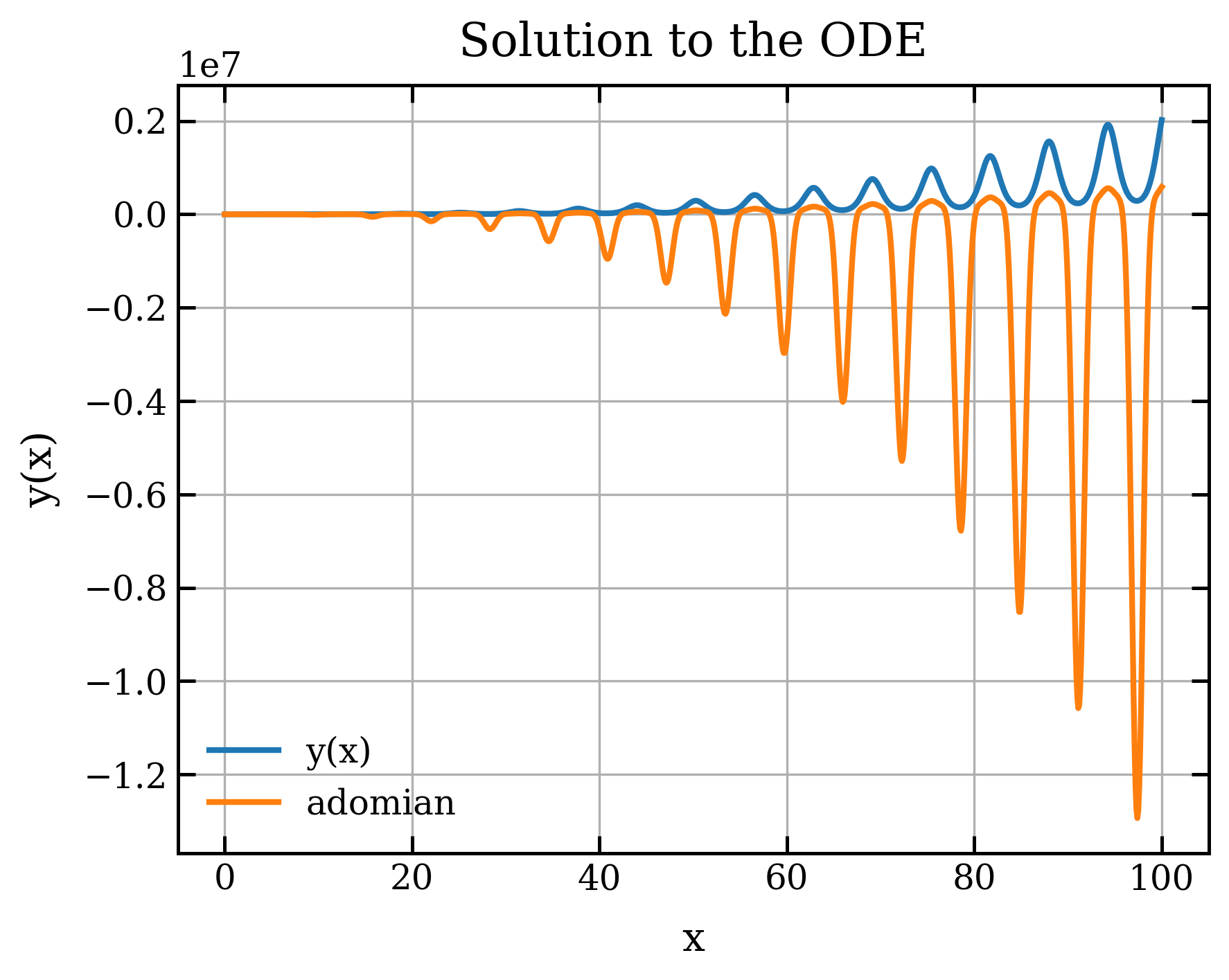
plt.plot(x_grid, solution, label="y(x)")
plt.plot(x_grid, adm(x_grid), label="adomian")
plt.xlabel("x")
plt.ylabel("y(x)")
plt.title("Solution to the ODE")
plt.legend()
plt.grid()
plt.savefig('figures/adomian_decomposition_solution.png', dpi=300, bbox_inches='tight')
plt.show()

Visualization

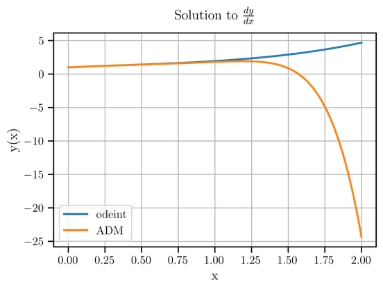
The following plot compares the Adomian decomposition solution with the numerical solution:

Linear 1 — worked example

Consider the following differential equation:

\frac{d y}{d x} + sin (x) y = 2 x^{2} + 1 y (0) = 3

We can substitute the P and Q values into the general expression along with our initial condition:

P (x) = sin (x)

Q (x) = 2 x^{2} + 1

This gives us the following iteration:

y_{0} (x) = 3 + \int_{0}^{x} (2 x^{2} + 1) d x

y_{k + 1} (x) = - \int_{0}^{x} sin (x) y_{k} (x) d x

Calculating the results of these iterations using a computer algebra system we get the following series. Note that the CAS was used to simplify each term, which resulted in a much shorter expression.

y_{0} = \frac{2 z ^{3}}{3} + z + 1

y_{1} = - \frac{2 z ^{3}}{3} - z + \frac{( 2 z ^{3} + 3 z + 3 ) cos ( z )}{3} - 1

y_{2} = (cos (z) - 1)^{2} (\frac{2 z ^{3}}{3} + z + 1)

y_{3} = (cos (z) - 1)^{3} (\frac{2 z ^{3}}{3} + z + 1)

y_{4} = (cos (z) - 1)^{4} (\frac{2 z ^{3}}{3} + z + 1)

Linear 1 worked example: Adomian decomposition vs numerical solution.

Reduced Riccati — recurrence derivation

The reduced Riccati equation is given by:

\frac{d y}{d x} = P (x) + Q (x) y^{2}

Integrating we find that:

y (x) = y (0) + \int_{0}^{x} P (x) d x + \int_{0}^{x} Q (x) y^{2} d x

The solution can be represented as a series:

y (x) = n = 0 \sum \infty y_{n} (x)

The nonlinear term can be represented as an Adomian Polynomial:

y^{2} = n = 0 \sum \infty A_{n} (x)

After substitution we are left with:

0 \sum \infty y_{n} (x) = y (0) + \int_{0}^{x} P (x) d x + \int_{0}^{x} Q (x) 0 \sum \infty A_{n} d x

Converting to recursive forms:

y_{0} (x) = y (0) + \int_{0}^{x} P (x) d x

y_{k + 1} (x) = \int_{0}^{x} Q (x) A_{k} d x

Future Directions

The following are extensions and adaptations to the standard method that I've thought about but haven't yet implemented or numerically validated. They're listed here as starting points for future work, not as documented techniques. Take everything below as conjecture until I (or you) actually build it.

Trapezoidal evaluation of Adomian integrals

One approach which could be used to facilitate the numerical calculation of the Adomian Decomposition is the use of the trapezoidal rule. In many cases the integrals which must be calculated become increasingly difficult to solve symbolically. To sidestep this, one could use the trapezoidal rule to evaluate them numerically. The trapezoidal rule does not extend the region of convergence — it just allows you to calculate the integral more easily. While the Adomian Decomposition does reduce the integration work compared to the Picard Iteration, the integrations can still rapidly become intractable.

Multi-stage Adomian

The Adomian Decomposition may only have a small radius of convergence. In this case it could be beneficial to apply the decomposition at different points along the domain.

v_{n + 1} (x) = \int_{x_{0}}^{x} A_{n} (s, v_{0} (s), v_{1} (s), ..., v_{n} (s)) d s

The basic idea is to develop an Euler-like method using the Adomian Decomposition on some small interval. We take our initial point and expand to the next point. We then apply the decomposition at the new initial condition and so on. One potential problem to be aware of is whether the multi-stage ADM is effective compared to an explicit Euler method — for small enough step sizes, the Adomian terms may collapse into a simple first-order extrapolation.

y_{k} + 1 \sum n v_{n} (x_{k} + h) = y_{k + 1}

Parameterized convergence control

One way to expand the region of convergence with the Adomian Decomposition might be to introduce a parameterized version of the method. The intuitive explanation: we can start iteration with any constant initial guess $c$ , then correct back using the term $v_{0} = y_{0} - c$ . The sum of the $v_{n}$ would still satisfy the boundary condition in this case, because $v_{0} + v_{1}$ equals the usual first iteration step in the Adomian iteration.

The proposed iteration:

v_{0} = y_{0} - c

v_{1} = c + \int_{x_{0}}^{x} f (x) d x

v_{n + 1} = \int_{x_{0}}^{x} v_{n} A_{n} d x

This parameterized version could also be combined with a multi-stage approach.

Automatic differentiation for convergence-control optimization

One difficulty with parameterized convergence control is that the method requires optimization of the series. The optimization can take many forms, but the result is that there are a set of parameters which need to be tuned for the method to work. This optimization could be handled with a traditional minimizer, but using an autograd framework one might be able to find a convergent series faster. The advantage of this is that in a multi-stage approach, parameters could be re-optimized rapidly at each step.

Padé aftertreatment

One feature of the Adomian Decomposition which can make it undesirable to use is that it does not extrapolate well. The same problem appears in a Taylor Series — after some distance the function wildly diverges. One potential solution is to compute the Padé approximant from the truncated Adomian series. My intuition is that this would help for most calculations: the Adomian Decomposition sometimes has a very small region of convergence, which makes it nearly impossible to use outside of a small step size. Without Padé aftertreatment, the asymptotic behavior will always be a divergence to positive or negative infinity. I haven't yet implemented this end-to-end.